Final Project

Welcome to your final project! This project is designed to bring together everything you’ve learned in this course, focusing on automating common MIKE+ modelling tasks using Python. You’ll prepare data, assess an existing model, and then perform a calibration exercise.

Project Specifications

Project Goal: To improve the performance of a sample MIKE+ model by calibrating catchment parameters using MIKE+Py for automation and ModelSkill for assessment.

Dataset:

You’ll be working with the Dyrup_uncalibrated model and associated rainfall and flow meter CSV data.

Download the project data: DyrupFinalProject_uncalibrated.zip

Ensure these files are in a data subfolder within your project directory. The Dyrup_uncalibrated.sqlite and .mupp files should be in the root of your project folder, or adjust paths in the code accordingly.

Your_Project_Folder/
├── data/
│   ├── rain_events.csv
│   └── station_flow_meters.csv
├── LTS/
│   └── rainfallBase.MJL
├── Dyrup_uncalibrated.sqlite
├── Dyrup_uncalibrated.mupp
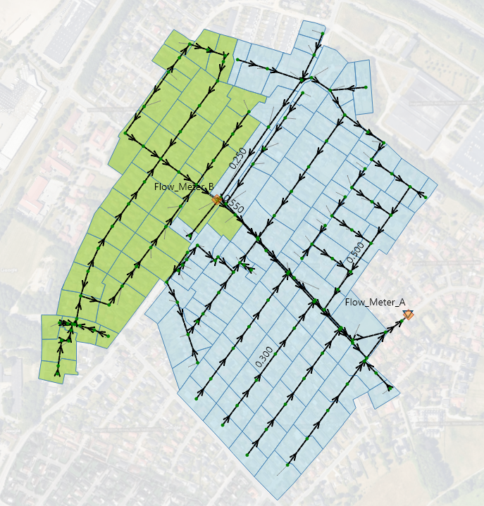
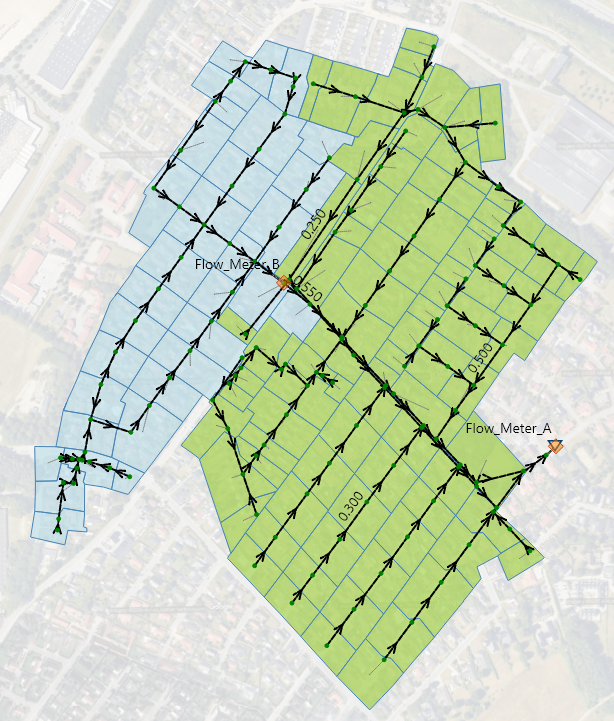
└── final_project.ipynb (or your script)

Familiarize yourself with the MIKE+ model before starting the project. It involves a storm sewer system using Model A with two flow meters: Flow Meter A (the outlet) and Flow Meter B. Flow Meter B drains into Flow Meter A. The model defines selections: one for areas draining to Flow Meter B and another for areas draining to Flow Meter A, excluding catchments from Flow Meter B.

Project Tracks:

Two tracks: Parts 1-3 are mandatory. Part 4 is an optional advanced challenge.

Standard Track (Mandatory):
- Part 1: Prepare rainfall and flow data.
- Part 2: Assess the skill of the existing, uncalibrated model.
- Part 3: Calibrate the model focusing on parameters affecting Flow Meter B.
Advanced Challenge (Optional):
- Part 4: Further calibrate the model, building upon Part 3, by focusing on parameters affecting Flow Meter A.

Let’s begin!

Install Python Packages

Install these required Python packages. Import necessary modules in your notebook.

uv pip install ipykernel pandas mikeio modelskill mikeplus mikeio1d matplotlib plotly nbformat

Part 1: Prepare Data

Objective: Convert rainfall and flow meter CSV data to dfs0 files.

Relevant Resources

Relevant Previous Exercises:

Module 2 Homework: CSV reading, Pandas processing, writing dfs0.

Tasks:

Process rainfall CSV to dfs0.

Starter Code: Task 1.1 - Process Rainfall Data

Remember to add necessary import statements at the beginning of your script/notebook. You may split this code into multiple cells.

# --- Part 1: Prepare Data ---
# Add imports (e.g., pandas, mikeio).

# Task 1.1: Rainfall CSV to dfs0

# 1. Load "data/rain_events.csv". Timestamps are in the first column (use as index, parse dates). Rainfall is µm/s.
# df_rain = ...

# 2. Define ItemInfo for the rainfall data.
#    - Name: "Rainfall Intensity"
#    - EUMType: Use mikeio.EUMType for Rainfall_Intensity.
#    - EUMUnit: Use mikeio.EUMUnit for mu_m_per_sec.
#    - data_value_type: "MeanStepBackward" (intensity over previous step).
# rainfall_item_info = ...

# 3. Convert df_rain to mikeio.Dataset using mikeio.from_pandas() and rainfall_item_info.
# ds_rain = ...

# 4. Save Dataset to "data/rain_events.dfs0" using .to_dfs().
# ...

Load rain_events.csv, ensuring dates are parsed correctly.
Convert the rainfall DataFrame to a MIKE IO Dataset.
- Define appropriate mikeio.ItemInfo (EUM type, unit, data value type, name).
Save the Dataset to data/rain_events.dfs0.

Process flow meter CSV to dfs0.

Starter Code: Task 1.2 - Process Flow Meter Data

Remember to add necessary import statements. You may split this code into multiple cells.

# Task 1.2: Flow meter CSV to dfs0

# 1. Load "data/station_flow_meters.csv". Timestamps in first column (use as index, parse dates). Discharge is m^3/s.
# df_flow_meters = ...

# 2. Define ItemInfo for Flow Meter A.
#    - Name: "Flow Meter A" (or your chosen column name).
#    - EUMType: Use mikeio.EUMType for Discharge.
#    - EUMUnit: Use mikeio.EUMUnit for meter_pow_3_per_sec.
#    - data_value_type: "Instantaneous".
# flow_meter_a_info = ...

# 3. Define ItemInfo for Flow Meter B (similarly).
# flow_meter_b_info = ... # Your code here

# 4. Convert flow meter DataFrame to mikeio.Dataset using a list of ItemInfo for both meters.
# ds_flow_meters = ... # Use mikeio.from_pandas()

# 5. Save Dataset to "data/station_flow_meters.dfs0".
# ...

Load station_flow_meters.csv, ensuring dates are parsed correctly.
Optionally, rename columns for clarity.
Convert the flow meter DataFrame to a MIKE IO Dataset.
- Define mikeio.ItemInfo for each flow meter (EUM type, unit, data value type, name).
Save the Dataset to data/station_flow_meters.dfs0.
Handle potential NaN values if present (though not expected for this dataset’s relevant period).

Checkpoint

Verify successful conversion of rainfall and flow data to dfs0.

rain_events.dfs0 created and contains one item with correct EUM type (Rainfall Intensity), unit (\(\mu m/s\)), and data value type (MeanStepBackward).
station_flow_meters.dfs0 created and contains two items, each with correct EUM type (Discharge), unit (\(m^3/s\)), and data value type (Instantaneous).

Part 2: Assess Skill of Existing Model

Objective: Run uncalibrated model, extract results, assess baseline skill with ModelSkill.

Relevant Resources

Relevant Previous Exercises:

Module 5 Homework: Running a simulation.
Module 3 Homework: Reading .res1d files, extracting data.
Module 4 Homework: Preparing data, matching, assessing skill with ModelSkill.

Tasks:

Run initial model.

Starter Code: Task 2.1 - Run Initial Model

Remember to add necessary import statements. You may split this code into multiple cells.

# --- Part 2: Assess Skill of Existing Model ---
# Add imports (e.g., mikeplus).

# Task 2.1: Run initial model
# Path to "Dyrup_uncalibrated.sqlite".
# initial_db_path = ... 

# 1. Open database with context manager.
# with ... as db:

# 2. Run simulation (MUID "rainfall"). db.run() returns list of Path objects.
# initial_result_files = ...

Open Dyrup_uncalibrated.sqlite with mikeplus.
Run the ‘rainfall’ simulation.
Store the paths to the generated result files.

Extract model results for ModelSkill.

Starter Code: Task 2.2 - Extract Model Results

Remember to add necessary import statements. You may split this code into multiple cells.

# Task 2.2: Extract model results
# Add imports (e.g., mikeio1d, mikeio, pandas).

# 1. Find network HD result file (e.g., "...Network_HD.res1d") from initial_result_files.
# hd_res1d_path_initial = ... 

# MUIDs for reaches: Flow Meter A ("G60F380_G60F360_l1"), B ("G62F070_G62F060_l1").
reach_fm_a = "G60F380_G60F360_l1"
reach_fm_b = "G62F070_G62F060_l1"

# 2. Open .res1d file with mikeio1d.open().
# res_initial = ...

# 3. Extract 'Discharge' for reach_fm_a. Save to "result_subsets/Model_FM_A_Initial.dfs0".
# res_initial.reaches[...].

# 4. Extract 'Discharge' for reach_fm_b. Save to "result_subsets/Model_FM_B_Initial.dfs0".
# res_initial.reaches[...].

Identify the network HD result file (e.g., ...Network_HD.res1d).
Open this file with mikeio1d.
Extract ‘Discharge’ for reaches G60F380_G60F360_l1 (Flow Meter A) and G62F070_G62F060_l1 (Flow Meter B).
Save extracted discharges to dfs0 files (e.g. result_subsets/Model_FM_A_Initial.dfs0)

Assess skill with ModelSkill.

Starter Code: Task 2.3 - Perform Skill Assessment

Remember to add necessary import statements. You may split this code into multiple cells.

# Task 2.3: Assess skill
# Add imports (e.g., modelskill, mikeio, pandas).

# Custom course metric defined for you (minimize for best performance).
# Use it the same way as other metrics, but DO NOT put its name in quotations.
from modelskill.metrics import metric, kge, pr

@metric(best="-") # Lower is better
def course_metric(obs, model):
    alpha = 0.5 # Weighting factor
    kge_val = kge(obs, model) 
    pr_val = pr(obs, model)
    kge_component = alpha * (1 - kge_val)
    pr_component = (1 - alpha) * abs(1 - pr_val)
    return kge_component + pr_component

# 1. Load observed flow data ("data/station_flow_meters.dfs0") to MIKE IO Dataset.
# ds_obs = ...

# 2. Load initial model results (e.g., "data/Model_FM_A_Initial.dfs0") to MIKE IO Datasets.
# ds_mod_a = ...
# ds_mod_b = ...

# 3. Create PointObservation for Flow Meter A from ds_obs. Use item name from Part 1. name="FM_A".
# obs_fm_a = ...

# 4. Create PointObservation for Flow Meter B similarly. name="FM_B".
# obs_fm_b = ...

# 5. Create PointModelResult for initial model output at FM A. name="MIKE+ Initial".
# mod_fm_a_initial = ...

# 6. Create PointModelResult for initial model output at FM B. name="MIKE+ Initial".
# mod_fm_b_initial = ...

# 7. Match obs_fm_a with mod_fm_a_initial using ms.match(max_model_gap=200).
# cmp_a_initial = ...

# 8. Match obs_fm_b with mod_fm_b_initial similarly.
# cmp_b_initial = ...

# 9. Create ComparerCollection from [cmp_a_initial, cmp_b_initial].
# cc_initial = ...

# 10. Plot cc_initial.plot.temporal_coverage().
# ...

# 11. For FM B (cmp_b_initial): plot scatter and timeseries(backend='plotly').
# ...

# 12. Skill table for cc_initial. Metrics: ['bias', 'rmse', 'nse', 'kge', 'pr', course_metric].
# metrics_to_calc = ['bias', 'rmse', 'nse', 'kge', 'pr', course_metric]
# skill_initial = ...

# 13. Mean skill table for cc_initial with same metrics.
# mean_skill_initial = ...

# 14. Review metrics: How is initial model performance?

Load observed flow data (data/station_flow_meters.dfs0).
Define and use the custom course_metric (referenced in code template).
Create ComparerCollection matching observations (Flow Meter A, B) with model results. Use max_model_gap=200.
Plot temporal coverage.
For Flow Meter B, generate scatter plot. Plot the time series using plotly as the backend, then explore.
Calculate and display skill tables (individual and mean) with ‘bias’, ‘rmse’, ‘nse’, ‘kge’, ‘pr’, and course_metric.
Reflect on the model’s existing skill, paying particular attention to kge, pr, and the course metric.

Checkpoint

Verify initial model run and baseline skill assessment.

Initial model results for FM A & B reaches saved to result_subsets/*.dfs0.
ComparerCollection created comparing initial model results with observed flow.
Baseline skill scores (esp. course_metric) for FM A and FM B.

Part 3: Calibrate Model

Objective: Calibrate ModelAConcTime & ModelARFactor for Flow Meter B catchments via grid search (MIKE+Py, ModelSkill).

What is a Grid Search?

A grid search runs the model for every combination of chosen parameter values. The best combination is based on a chosen metric (e.g., course_metric). See Wikipedia: Grid search.

Relevant Resources

Relevant Previous Exercises:

Module 5 Homework: Selecting data, creating scenarios/alternatives, looping, modifying parameters, running simulations (especially Exercise 5).
Module 4 Homework: As in Part 2 for ModelSkill.

Tasks:

Setup calibration for FM B.

Starter Code: Task 3.1 - Setup for Calibration (FM B)

Remember to add necessary import statements. You may split this code into multiple cells.

# --- Part 3: Calibrate Model at Flow Meter B ---
# Add imports (e.g., numpy, mikeplus).

# Task 3.1: Set up for calibration

# 1. Open database. Query "m_Selection" for "ItemMUID" where "SelectionID" is "Flow_Meter_B_Catchments" AND "TableName" is "msm_Catchment". Store MUIDs in catchments_b_muids list.
# with ... as db:
    # selection_df = (db.tables.m_Selection
                    # .select(...) # Select "ItemMUID"
                    # .where(...) # Filter by SelectionID
                    # .where(...) # Filter by TableName
                    # .to_dataframe())
    # catchments_b_muids = selection_df["ItemMUID"].tolist()

# 2. Review ModelAConcTime & ModelARFactor for catchments_b_muids. Query "msm_Catchment", filter by MUIDs, describe().
# with ... as db: # Or reuse open db if still in context

# 3. Define parameter ranges for Tc (Time of Conc.) and R_factor (Reduction Factor) using np.linspace() (e.g., 3 values each).
# tc_vals_b = ...
# r_vals_b = ...

Open Dyrup_uncalibrated.sqlite.
Retrieve MUIDs for catchments in selection “Flow_Meter_B_Catchments”.
Review existing Time of Concentration (Tc) and Reduction Factor (R_factor) for these catchments.
Define ranges for Tc and R_factor for these catchments (e.g., 3 values for each parameter to create a 3x3 grid).

Grid parameters apply to all catchments in the “Flow_Meter_B_Catchments” group.

Long Runtimes

Running many MIKE+ simulations can be time-consuming. It’s suggested to keep the grid search low initially (e.g. 3x3 = 9 trials). Once your workflow is defined, and you want to refine the calibration, then consider creating more trials.

Single calibration trial (FM B).

Starter Code: Task 3.2 - Perform a Single Calibration Trial (FM B)

Add necessary imports.

# Task 3.2: Single trial (FM B)

# 1. Pick one Tc and one R_factor from defined ranges.
# tc_trial = tc_vals_b[0]  # Example: first Tc value
# r_factor_trial = r_vals_b[0] # Example: first R_factor value

# 2. Define unique name for alternative & scenario (use f-string with param values).
# name = f"Trial 0 (tc={tc:.0f}, r={r_factor:.3f})"

# 3. Create alternative & scenario. Activate scenario. Verify in MIKE+.
# with ... as db:
#    alt_group = db.alternative_groups[...]
#    alternative = alt_group.create(...)
#    scenario = db.scenarios.create(...)
#    scenario.set_alternative(...)
#    scenario.activate()

# 4. Update ModelAConcTime & ModelARFactor for catchments_b_muids. Execute & verify.
# updated = (
#   db.tables.msm_Catchment
#     .update({...}) # Define columns and new values
#     .by_muid(...)  # Specify MUIDs to update
#     .execute()
# )
# len(updated)

# 5. Update 'rainfall' sim setup in msm_Project to use new scenario.
# (db.tables.msm_Project
#     .update({...}) # Define column and new value
#     .by_muid(...)  # Specify simulation MUID
#     .execute())

# 6. Run the 'rainfall' simulation and store the list of result file Paths.
# result_files = db.run(...)

# 7. Open .res1d with mikeio1d.
# res_single_trial = ...

# 8. Extract Discharge for FM B to dfs0.
# ...

# 9. Create PointModelResult. Name it like scenario/alternative (trial_name).
# mod_result_single_trial = ms.PointModelResult(...)

# 10. Match with obs_fm_b.
# comparer_single_trial = ms.match(...)

# 11. Plot scatter & timeseries (as in Part 2).
# ...

# 12. Calculate skill (include course_metric).
# skill_single_trial = comparer_single_trial.skill(...)

# 13. Review metrics: How does this trial compare with the initial model?

This task guides you to run one iteration of the calibration process. This will help you understand the steps involved before automating them in a loop for the entire grid search.

Work on the database Dyrup_uncalibrated.sqlite.
Perform all steps for one parameter combination: create scenario/alternative, update parameters, run simulation, extract results, calculate course_metric.
Verify that the process works and compare the output metric with the initial model’s metric for Flow Meter B.

Automated grid search (FM B).

Starter Code: Task 3.3 - Automated Grid Search (FM B)

Remember to add necessary import statements.

# Task 3.3: Automated grid search (FM B)
# import itertools

# Store results: trial_name -> hd_res1d_path
trial_b_results = {}   

# 1. Open database ONCE for the loop (context manager).
# with ... as db:

    # 2. Get alternative group for "Catchments and hydrology data".
    # alt_group = db.alternative_groups[...]

    # 3. Loop all Tc & R_factor combinations (itertools.product).
    # for i, (tc, r_factor) in enumerate(itertools.product(tc_vals_b, r_vals_b), start=1):
        # print(f"Starting Trial {i}: Tc={tc_current:.0f}, R_factor={r_current:.2f}")

        # 4. Define unique alt/scenario name.
        # trial_name = f"Trial {i} (tc={tc:.0f}, r={r_factor:.3f})"

        # 5. Create & activate new alt/scenario.
        # ...

        # 6. Update catchment Tc & R_factor for catchments_b_muids.
        # ...

        # 7. Update msm_Project, run simulation, get HD result file path.
        # ...

        # 8. Store HD result path in trial_b_results.
        # trial_b_results[trial_name] = ...

Using the database Dyrup_uncalibrated.sqlite, loop through all combinations of Tc and R_factor.
Inside the loop, include all the steps to create a scenario/alternative, update parameters for the current Tc and R_factor, and run the simulation.
Save the result of the loop in a dictionary, with keys being the scenario name and values being the path to the res1d result file.
Open MIKE+, activate a few scenarios, and check the parameters to ensure your code worked as intended.

Caution

Test your code carefully before running it in the full loop. Use cells to test chunks of code. If you accidentally destroy the model database, it’s easiest to start over with a fresh copy of the database. Luckily you have a reproducible workflow that’s as easy as running all cells :).

Analyze calibration results (FM B).

Starter Code: Task 3.4 - Analyze Calibration Results (FM B)

Remember to add necessary import statements. You may split this code into multiple cells.

# Task 3.4: Analyze FM B calibration results

# 1. Loop over `trial_b_results` from the previous part. Create a list of comparer objects at Flow Meter B for each trial.
# comparers = []
# for scenario_name, res1d_path in trial_b_results.items():
#     res = mikeio1d.open(res1d_path)
#     ... some more code to get result data into modelskill
#     cmp = ms.match(...)
#     comparers.append(cmp)

# 2. Add the comparer object from MIKE+ Initial at Flow Meter B
# comparers.append(...)

# 3. Create a ComparerCollection of all the trials and the initial model.
# cc_fm_b = ms.ComparerCollection(...)

# 4. Save the ComparerCollection so that you can reload it in the future.
# cc_fm_b.save("flow_meter_b_calibration.msk") 
# cc_fm_b = cc_fm_b.load("flow_meter_b_calibration.msk") # this is how you would load it

# 5. Skill table for cc_fm_b (include course_metric).
# skill_fm_b = cc_fm_b.skill(...)

# 6. Sort skill_fm_b by course_metric to find best/worst trials. Display styled table.
# skill_fm_b

# 7. Plot best and worst trials vs. MIKE+ Initial (e.g., scatter, timeseries for FM B).
# cc_fm_b[0].sel(model=["MIKE+ Initial", ...]).plot.

# 8. Review metrics: How do these trials compare?

Create a ComparerCollection for Flow Meter B:
- Include the “MIKE+ Initial” model results (from Part 2).
- Include all trials from the previous part..
(Optional: save/load .msk file).
Calculate the skill table for Flow Meter B using course_metric and other standard metrics.
Sort the skill table to find the best and worst trials, according to course_metric.
Make plot comparisons of the best trial versus MIKE+ Initial to support the calibration efforts.

Checkpoint

Verify automated calibration for FM B and result analysis.

Dyrup_uncalibrated.sqlite contains all scenarios/alternatives for FM B grid search.
All grid search sim result files generated (or best trial’s .res1d path is known).
Best ModelAConcTime & ModelARFactor for FM B catchments identified via course_metric.
Performance improvement at FM B quantified (using course_metric) and visualized.

Part 4: More Calibration (optional)

Objective: Further calibrate for Flow Meter A catchments. Use Part 3’s best scenario as parent.

Tasks:

There’s no code templates or checkpoints for this part - you’re on your own :)
Repeat Part 3 process for FM A catchments.
Create functions to reuse Part 3 code (recommended).
Create ComparerCollection for FM A & B. Calculate overall mean course_metric.