Show Plotting Code
ax = df.plot()
ax.axvspan(
    xmin="1993-12-06 00:00",
    xmax="1993-12-07 00:00",
    color='grey',
    alpha=0.3,
    label="Missing Data"
)
ax.legend(loc="upper right")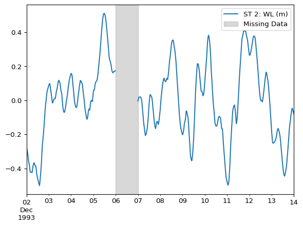
Data cleaning is an essential step in any MIKE+ modelling workflow to ensure your input data is complete. This section covers handling missing values (e.g. nan). Additionally, it introduces the topic of detecting anomalies in time series data.
DHI’s modelling engines typically require complete datasets for calculations, and thus dfs0 files, which are often used as inputs, should not contain missing values. For example, a rainfall boundary condition cannot have the value nan.
Missing numerical data is typically represented by nan. These arise from various sources, such as sensor malfunctions during data collection, gaps that occur during data transmission, or they might be the result of previous data processing or cleaning steps.
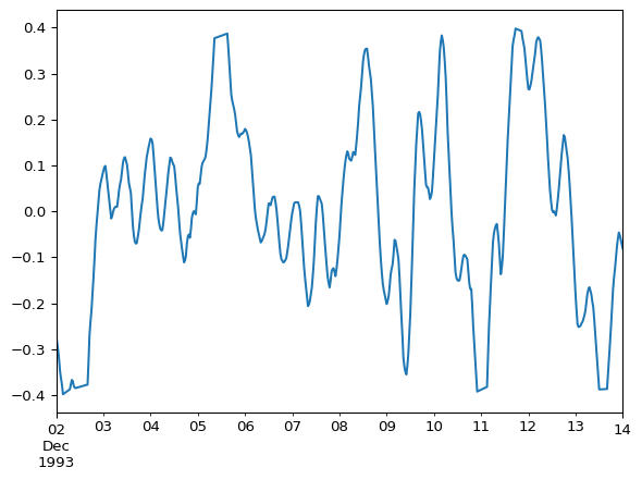
Assume we have a DataFrame with missing values on 1993-12-06:
ax = df.plot()
ax.axvspan(
xmin="1993-12-06 00:00",
xmax="1993-12-07 00:00",
color='grey',
alpha=0.3,
label="Missing Data"
)
ax.legend(loc="upper right")
Count the number of missing values (e.g. nan) for each time series by summing the result of isna().
df.isna().sum()ST 2: WL (m) 48
dtype: int64The process of filling missing values is known as imputation.
For missing values between valid data points (i.e. bounded), using the .interpolate() method is a common and effective approach.
df_interpolated = df.interpolate(method='time')ax = df.plot()
ax.axvspan(
xmin="1993-12-06 00:00",
xmax="1993-12-07 00:00",
color='grey',
alpha=0.3,
label="Missing Data"
)
df_interpolated.columns = ["Interpolation"]
df_interpolated.loc["1993-12-06"].plot(ax=ax)
ax.legend(loc="upper right")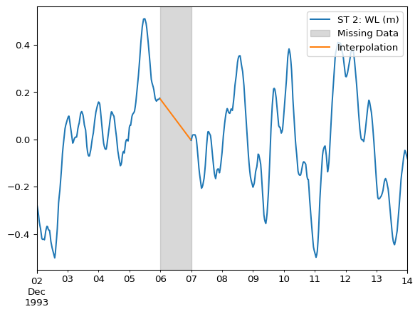
The example above uses method='time', which is a linear interpolation that considers non-equidistant DatetimeIndex indices. Refer to Pandas’s documentation for additional interpolation methods, such as polynomial.
For missing values appearing at the very beginning or end of your dataset (i.e. unbounded), you can make use of:
.fillna().ffill().bfill()Recall: these imputation methods were introduced in the section on resampling, where upsampling introduced nan values.
Same example as above, but using ffill().
df_interpolated = df.ffill()ax = df.plot()
ax.axvspan(
xmin="1993-12-06 00:00",
xmax="1993-12-07 00:00",
color='grey',
alpha=0.3,
label="Missing Data"
)
df_interpolated.columns = ["Interpolation"]
df_interpolated.loc["1993-12-06"].plot(ax=ax)
ax.legend(loc="upper right")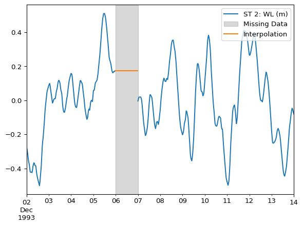
Same example as above, but using bfill().
df_interpolated = df.bfill()ax = df.plot()
ax.axvspan(
xmin="1993-12-06 00:00",
xmax="1993-12-07 00:00",
color='grey',
alpha=0.3,
label="Missing Data"
)
df_interpolated.columns = ["Interpolation"]
df_interpolated.loc["1993-12-06"].plot(ax=ax)
ax.legend(loc="upper right")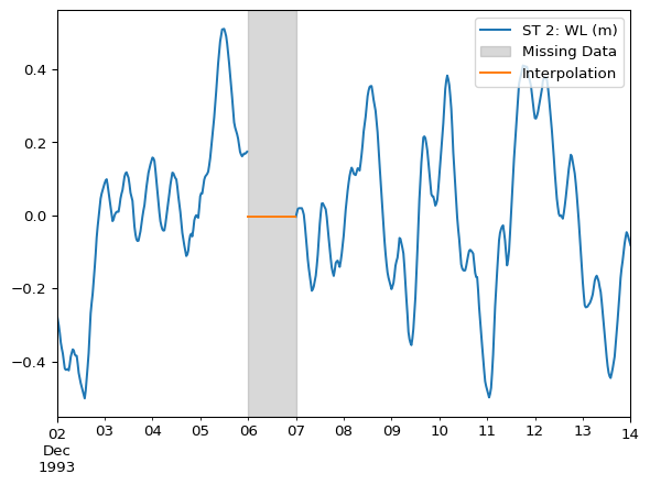
Same example as above, but using fillna().
df_interpolated = df.fillna(0.1) # specify the value to fill withax = df.plot()
ax.axvspan(
xmin="1993-12-06 00:00",
xmax="1993-12-07 00:00",
color='grey',
alpha=0.3,
label="Missing Data"
)
df_interpolated.columns = ["Interpolation"]
df_interpolated.loc["1993-12-06"].plot(ax=ax)
ax.legend(loc="upper right")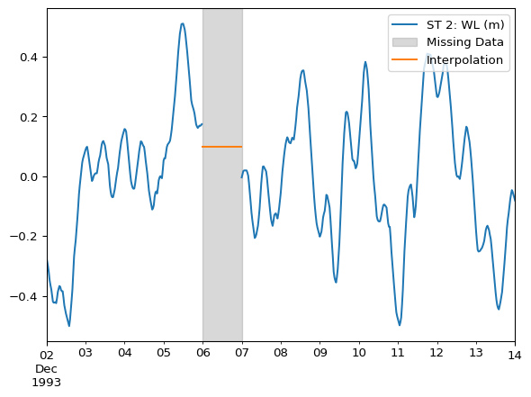
Short on time? This section provides an introduction to a useful package but can be considered optional for core module understanding.
Beyond clearly missing values, time series data can also contain anomalies. Identifying and addressing these anomalies is crucial for building robust MIKE+ models.
Anomaly detection is a broad and complex field. This section offers a basic introduction to rule-based anomaly detection using DHI’s tsod Python package.
uv pip install tsodtsod operates using a concept called “detectors.” Each detector is designed to implement a specific rule or heuristic to identify anomalies. Example anomaly detectors:
RangeDetector: Flags values outside a set range.ConstantValueDetector: Detects unchanging values over time.DiffDetector: Catches large changes between points.RollingStdDetector: Finds points far from rolling standard deviation.There’s also the CombinedDetector, which allows combining the rules of several detectors.
Plot the initial time series.
ts = df["ST 2: WL (m)"]
ts.plot()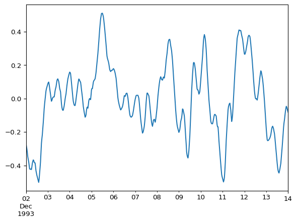
tsod operates on Series. Select the subject Series from the DataFrame object as needed.
Select and instantiate a detector. If we know water levels must be in the range -0.4m to 0.4m, then a RangeDetector should be used.
from tsod.detectors import RangeDetector

detector = RangeDetector(
    min_value = -0.4,
    max_value = 0.4
)
detector
RangeDetector(min: -4.0e-01, max: 4.0e-01)Detect anomalies for a given Series using the detect() method of the instantiated detector.
anomaly_mask = detector.detect(ts)
anomaly_mask.head()
1993-12-02 00:00:00 False
1993-12-02 00:30:00 False
1993-12-02 01:00:00 False
1993-12-02 01:30:00 False
1993-12-02 02:00:00 False
Freq: 30min, Name: ST 2: WL (m), dtype: boolA mask refers to a boolean indexer. In the example above, values are true for anomalies and false otherwise.
Plot the detected anomalies.
ax = ts.plot()
ts[anomaly_mask].plot(
    ax=ax,
    style='ro',
    label="Anomaly",
    alpha=0.5
)
ax.legend()

# horizontal lines to validate ranges
ax.axhline(0.4, color='grey', alpha=0.5)
ax.axhline(-0.4, color='grey', alpha=0.5)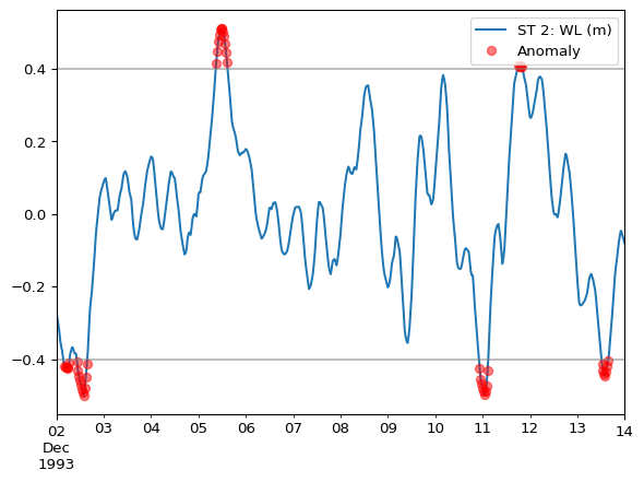
Replace anomalies with nan.
import numpy as np

ts_cleaned = ts.copy()
ts_cleaned[anomaly_mask] = np.nan
ts_cleaned.plot()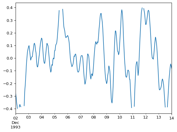
Impute anomalies by treating them just like missing values.
ts_cleaned = ts_cleaned.interpolate(method='time')
ts_cleaned.plot()