11  Data Selection

This section explores how to select specific subsets of time series data.

11.1 Why subset data?

Selecting a subset of data is useful for:

  • focusing analysis on data of interest (e.g. specific item or time range)
  • reducing memory usage and computational overhead (helpful for large files)
  • generating relevant illustrations (plots and table views)

11.2 Alternative Methods

There are various ways of selecting subsets of dfs0 data. This section covers two different approaches:

  1. Using mikeio.read()
  2. Using Pandas DataFrame

As mentioned, MIKE IO also provides additional functionality for selecting subsets, however this course focuses on Pandas for simplicity.

Selecting data via the read() method is generally most performant, since it will avoid loading the entire file into memory. Selecting data via Dataset, DataArray, and DataFrame objects requires first loading the entire file into memory.

A dfs0 file is a special case where the entire file is loaded into memory regardless, however that will not be the case for other dfs formats (e.g. dfs2, dfsu). Therefore, it’s a good practice to use the read() method when you know which data you want in advance.

11.3 Selecting Items

When reading data with mikeio.read(), the items argument lets you specify which items to load. You can do this by providing a list of item names.

ds = mikeio.read(
    "data/sirius_idf_rainfall.dfs0", 
    items=[" F=1", " F=2"]
)
ds
<mikeio.Dataset>
dims: (time:22)
time: 2019-01-01 00:00:00 - 2019-01-02 00:00:00 (22 non-equidistant records)
geometry: GeometryUndefined()
items:
  0:   F=1 <Rainfall Intensity> (mm per hour) - 3
  1:   F=2 <Rainfall Intensity> (mm per hour) - 3

Alternatively, you can select items using their numerical indices (zero-based). For example, to load the first and third items:

ds = mikeio.read(
    "data/sirius_idf_rainfall.dfs0",
    items=[4, 3]
)
ds
<mikeio.Dataset>
dims: (time:22)
time: 2019-01-01 00:00:00 - 2019-01-02 00:00:00 (22 non-equidistant records)
geometry: GeometryUndefined()
items:
  0:   F=1 <Rainfall Intensity> (mm per hour) - 3
  1:   F=2 <Rainfall Intensity> (mm per hour) - 3
Tip

Using item indices can be convenient, especially for quick explorations. However, specifying item names explicitly makes your code more readable and robust to changes in the dfs0 file structure, such as if items are reordered.

From a Pandas DataFrame, you can select items using standard Pandas column selection techniques.

ds = mikeio.read("data/sirius_idf_rainfall.dfs0")
df = ds.to_dataframe()
df.head()
F=20 F=10 F=5 F=2 F=1 F=0.5 F=0.2 F=0.1 F=0.05
2019-01-01 00:00:00 0.00 0.000000 0.0 0.0 0.000000 0.000000 0.000000 0.000000 0.0
2019-01-01 06:00:00 0.15 0.283333 0.4 0.4 0.466667 0.683333 0.966667 1.316667 1.4
2019-01-01 07:00:00 0.20 0.400000 0.6 0.6 0.800000 1.100000 1.600000 2.200000 2.3
2019-01-01 08:00:00 0.30 0.600000 0.7 0.8 0.900000 1.400000 2.000000 2.800000 3.1
2019-01-01 09:00:00 0.30 0.600000 0.9 1.0 1.200000 1.800000 2.600000 3.600000 4.0

To select a single item:

df[[" F=20"]].head()
F=20
2019-01-01 00:00:00 0.00
2019-01-01 06:00:00 0.15
2019-01-01 07:00:00 0.20
2019-01-01 08:00:00 0.30
2019-01-01 09:00:00 0.30
Tip

Indexing with a list returns another DataFrame, whereas indexing with a single value returns a Series.

For multiple items, provide a list of column names:

df[[" F=1", " F=2"]].head()
F=1 F=2
2019-01-01 00:00:00 0.000000 0.0
2019-01-01 06:00:00 0.466667 0.4
2019-01-01 07:00:00 0.800000 0.6
2019-01-01 08:00:00 0.900000 0.8
2019-01-01 09:00:00 1.200000 1.0

11.4 Selecting Time Steps

When reading data with mikeio.read(), the time argument allows for various ways to specify the desired subset.

You can select by a single time step index (e.g., the first time step, index 0).

ds = mikeio.read(
    "data/single_water_level.dfs0",
    time=0
)
ds
<mikeio.Dataset>
dims: ()
time: 1993-12-02 00:00:00 (time-invariant)
geometry: GeometryUndefined()
items:
  0:  ST 2: WL (m) <Water Level> (meter)

Or provide a list of indices for specific time steps (e.g., the first three time steps).

ds = mikeio.read(
    "data/single_water_level.dfs0",
    time=[0,1,2]
)
ds
<mikeio.Dataset>
dims: (time:3)
time: 1993-12-02 00:00:00 - 1993-12-02 01:00:00 (3 records)
geometry: GeometryUndefined()
items:
  0:  ST 2: WL (m) <Water Level> (meter)

You can also use timestamp strings.

ds = mikeio.read(
    "data/single_water_level.dfs0",
    time="1993-12-02 00:00:00"
)
ds
<mikeio.Dataset>
dims: ()
time: 1993-12-02 00:00:00 (time-invariant)
geometry: GeometryUndefined()
items:
  0:  ST 2: WL (m) <Water Level> (meter)

Select multiple timestamps with a more general string, such as all times on a specific date.

ds = mikeio.read(
    "data/single_water_level.dfs0",
    time="1993-12-03"
)
ds
<mikeio.Dataset>
dims: (time:48)
time: 1993-12-03 00:00:00 - 1993-12-03 23:30:00 (48 records)
geometry: GeometryUndefined()
items:
  0:  ST 2: WL (m) <Water Level> (meter)

To specify a time range, use Python’s slice() object with start and end timestamps:

ds = mikeio.read(
    "data/single_water_level.dfs0",
    time=slice("1993-12-02 12:00", "1993-12-02 16:00")
)
ds
<mikeio.Dataset>
dims: (time:9)
time: 1993-12-02 12:00:00 - 1993-12-02 16:00:00 (9 records)
geometry: GeometryUndefined()
items:
  0:  ST 2: WL (m) <Water Level> (meter)
Tip

Python’s slice() method is versatile for defining ranges. While list-like slicing notation (e.g., time_series[start:end]) is common with Pandas DataFrames, slice(start, end) is the explicit way to create a slice object, often used in functions like mikeio.read().

From a Pandas DataFrame, standard indexing and slicing techniques of the DatetimeIndex may be used.

To select by time step index, use .iloc.

ds = mikeio.read("data/single_water_level.dfs0")
df = ds.to_dataframe()
df.iloc[[0]] 
ST 2: WL (m)
1993-12-02 -0.2689
Tip

Providing a list to iloc returns another DataFrame, whereas providing a single value returns a Series.

For the first three time steps:

df.iloc[0:3]
ST 2: WL (m)
1993-12-02 00:00:00 -0.2689
1993-12-02 00:30:00 -0.2847
1993-12-02 01:00:00 -0.3020

For selection by timestamp strings, use .loc.

df.loc[["1993-12-02 00:00:00"]]
ST 2: WL (m)
1993-12-02 -0.2689

To select all data for a particular day:

df.loc["1993-12-03"].head()
ST 2: WL (m)
1993-12-03 00:00:00 0.0879
1993-12-03 00:30:00 0.0951
1993-12-03 01:00:00 0.0988
1993-12-03 01:30:00 0.0836
1993-12-03 02:00:00 0.0634

And for a range between start and end timestamps:

df.loc["1993-12-02 12:00":"1993-12-02 16:00"]
ST 2: WL (m)
1993-12-02 12:00:00 -0.4590
1993-12-02 12:30:00 -0.4698
1993-12-02 13:00:00 -0.4812
1993-12-02 13:30:00 -0.4919
1993-12-02 14:00:00 -0.5012
1993-12-02 14:30:00 -0.4798
1993-12-02 15:00:00 -0.4486
1993-12-02 15:30:00 -0.4137
1993-12-02 16:00:00 -0.3772

A key distinction in Pandas is between .iloc and .loc:

  • .iloc is used for integer-location based indexing (by position, e.g., df.iloc[0] for the first row).
  • .loc is used for label-based indexing (by index names or boolean arrays, e.g., df.loc['2023-01-01']).

When working with time series data having a DatetimeIndex, .loc is particularly powerful as it allows you to use date/time strings for intuitive selections and slicing, as shown in the examples.
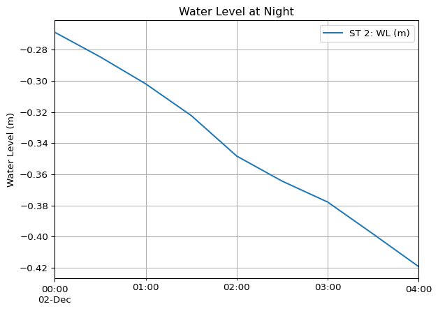
11.5 Example

Let’s tie these concepts together with an example of plotting a subset of a dfs0 file.

1. Read a specific item of the dfs0 file into a Dataset

ds = mikeio.read("data/single_water_level.dfs0", items="ST 2: WL (m)")
ds
<mikeio.Dataset>
dims: (time:577)
time: 1993-12-02 00:00:00 - 1993-12-14 00:00:00 (577 records)
geometry: GeometryUndefined()
items:
  0:  ST 2: WL (m) <Water Level> (meter)

2. Convert to Pandas DataFrame:

df = ds.to_dataframe()
df
ST 2: WL (m)
1993-12-02 00:00:00 -0.2689
1993-12-02 00:30:00 -0.2847
1993-12-02 01:00:00 -0.3020
1993-12-02 01:30:00 -0.3223
1993-12-02 02:00:00 -0.3483
... ...
1993-12-13 22:00:00 -0.0462
1993-12-13 22:30:00 -0.0522
1993-12-13 23:00:00 -0.0619
1993-12-13 23:30:00 -0.0717
1993-12-14 00:00:00 -0.0814

577 rows × 1 columns

3. Filter the Pandas DataFrame for the time range of interest.

df = df.loc["1993-12-02 00:00":"1993-12-02 4:00"]
df
ST 2: WL (m)
1993-12-02 00:00:00 -0.2689
1993-12-02 00:30:00 -0.2847
1993-12-02 01:00:00 -0.3020
1993-12-02 01:30:00 -0.3223
1993-12-02 02:00:00 -0.3483
1993-12-02 02:30:00 -0.3644
1993-12-02 03:00:00 -0.3778
1993-12-02 03:30:00 -0.3983
1993-12-02 04:00:00 -0.4192

4. Plot

ax = df.plot()
ax.set_title("Water Level at Night")
ax.set_ylabel("Water Level (m)")
ax.grid(which="both")

Tip

Plot methods often return a Matplotlib Axes object, conventionally called ax. Use it to customize the plot before it’s displayed a Jupyter Cell.