df.head()| ST 2: WL (m) | |
|---|---|
| 1993-12-02 00:00:00 | -0.2689 |
| 1993-12-02 00:30:00 | -0.2847 |
| 1993-12-02 01:00:00 | -0.3020 |
| 1993-12-02 01:30:00 | -0.3223 |
| 1993-12-02 02:00:00 | -0.3483 |
Resampling is a powerful technique for changing the frequency of time series data, a common task when working with MIKE+ model inputs or outputs.
At its core, resampling involves adjusting the time steps in your data. There are two main types:
A prerequisite for resampling in Pandas is that the DataFrame must have a DatetimeIndex. This will be the case if it was created via MIKE IO’s to_dataframe() method.
If a DataFrame’s index is time-like but not already a DatetimeIndex, you can usually convert it with:
df.index = pd.to_datetime(df.index)Two common motivations for resampling time series data in MIKE+ modelling are:
Pandas provides a straightforward resample() method for time series data.
The general syntax is: df.resample(<rule>).<aggregation_or_fill_method>().
.mean() or .sum(). For upsampling, this is a fill method like .ffill() or .interpolate().
A quick example for illustration with the following DataFrame:
df.head()| ST 2: WL (m) | |
|---|---|
| 1993-12-02 00:00:00 | -0.2689 |
| 1993-12-02 00:30:00 | -0.2847 |
| 1993-12-02 01:00:00 | -0.3020 |
| 1993-12-02 01:30:00 | -0.3223 |
| 1993-12-02 02:00:00 | -0.3483 |
To resample this half-hourly data to daily mean values:
df_daily_mean = df.resample('D').mean()
df_daily_mean.head()| ST 2: WL (m) | |
|---|---|
| 1993-12-02 | -0.302979 |
| 1993-12-03 | 0.041185 |
| 1993-12-04 | 0.014558 |
| 1993-12-05 | 0.265933 |
| 1993-12-06 | -0.004035 |
ax = df.plot()
df_daily_mean.plot(ax=ax)
ax.legend(["Original", "Downsampled"])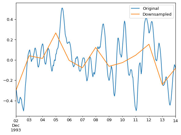
Pandas offers many frequency aliases (rules). Some of the most common include:
"M": Month-end frequency"W": Weekly frequency (defaults to Sunday)"D": Calendar day frequency"H": Hourly frequency"15min": 15-minute frequencyFor a comprehensive list of frequency strings (offset aliases), refer to the Pandas documentation on Time Series / Date functionality.
When downsampling, you are reducing the number of data points, so you need to decide how to aggregate the values within each new, larger time period. Common aggregation methods include:
.mean(): calculate the average of the values..sum(): calculate the sum of the values..first(): select the first value in the period..last(): select the last value in the period..min(): find the minimum value..max(): find the maximum value.The choice of aggregation method depends on the nature of your data and what you want to represent. For instance, rainfall is often summed, while water levels or flows might be averaged.
Resample to daily values by choosing the maximum value on each day.
df_daily_max = df.resample('D').max()
df_daily_max.head()| ST 2: WL (m) | |
|---|---|
| 1993-12-02 | 0.0799 |
| 1993-12-03 | 0.1486 |
| 1993-12-04 | 0.1583 |
| 1993-12-05 | 0.5106 |
| 1993-12-06 | 0.1793 |
Or, choose the minimum value on each day.
df_daily_min = df.resample('D').min()
df_daily_min.head()| ST 2: WL (m) | |
|---|---|
| 1993-12-02 | -0.5012 |
| 1993-12-03 | -0.0701 |
| 1993-12-04 | -0.1112 |
| 1993-12-05 | 0.0524 |
| 1993-12-06 | -0.1114 |
Compare these two aggregation methods with a plot.
ax = df.plot(color='grey')
df_daily_mean.plot(ax=ax, linestyle="--")
df_daily_min.plot(ax=ax, linestyle="--")
df_daily_max.plot(ax=ax, linestyle="--")
ax.legend(["Original", "Downsample (mean)", "Downsample (min)", "Downsample (max)"])
ax.grid(which="both")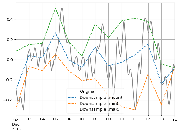
When upsampling, you are increasing the number of data points, which means you’ll have new time steps with no existing data. You need to specify a method to fill these gaps. Common fill methods include:
.ffill() (forward fill): propagate the last valid observation forward..bfill() (backward fill): use the next valid observation to fill the gap..interpolate(): fill nan values using an interpolation method (e.g., linear, spline).nan stands for ‘not a number’, which is a common way to represent missing values. See NumPy’s nan.
Recall our original DataFrame had half-hourly time steps:
df.head(2) # show only first two rows| ST 2: WL (m) | |
|---|---|
| 1993-12-02 00:00:00 | -0.2689 |
| 1993-12-02 00:30:00 | -0.2847 |
Upsample this to a resolution of one minute, comparing ffill and bfill:
df.resample("5min").ffill().head()| ST 2: WL (m) | |
|---|---|
| 1993-12-02 00:00:00 | -0.2689 |
| 1993-12-02 00:05:00 | -0.2689 |
| 1993-12-02 00:10:00 | -0.2689 |
| 1993-12-02 00:15:00 | -0.2689 |
| 1993-12-02 00:20:00 | -0.2689 |
df.resample("5min").bfill().head()| ST 2: WL (m) | |
|---|---|
| 1993-12-02 00:00:00 | -0.2689 |
| 1993-12-02 00:05:00 | -0.2847 |
| 1993-12-02 00:10:00 | -0.2847 |
| 1993-12-02 00:15:00 | -0.2847 |
| 1993-12-02 00:20:00 | -0.2847 |
Compare the difference between these two. Find the new time stamps and how their values were chosen.
Depending on use case, a more appropriate approach may be filling gaps with linear interpolation:
df_interpolated = df.resample('5min').interpolate(method='linear')
df_interpolated.head()| ST 2: WL (m) | |
|---|---|
| 1993-12-02 00:00:00 | -0.268900 |
| 1993-12-02 00:05:00 | -0.271533 |
| 1993-12-02 00:10:00 | -0.274167 |
| 1993-12-02 00:15:00 | -0.276800 |
| 1993-12-02 00:20:00 | -0.279433 |
Compare interpolation to original data for a zoomed-in time period:
subset = slice("1993-12-02 00:00:00", "1993-12-02 08:00:00")
ax = df.loc[subset].plot(color="grey", alpha=0.7, linewidth=8)
df_interpolated.loc[subset].plot(ax=ax, linestyle="--")
ax.legend(["Original", "Interpolated"])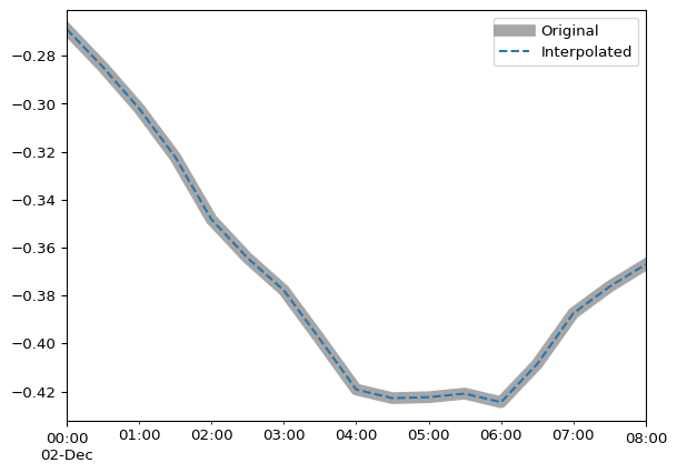
Upsampling should be done with caution, as it involves making assumptions about the data between known points. The choice of fill method can significantly impact the resulting time series.