This section covers how to select specific subsets of network result data.
19.1 Alternative Methods
There are various ways of selecting subsets of network result data. This section covers three main approaches:
Using Pandas DataFrame.
Using the Res1D object to subset locations and quantities.
Using mikeio1d.open().
Memory considerations
Similar to MIKE IO, selecting data via open() is generally most performant since it avoids loading the entire file into memory.
19.2 Selecting Locations
When dealing with network results, you often want to focus on specific parts of your model, like certain nodes or reaches.
Selecting data purely with DataFrames can be difficult due to the large number of columns and their header format. For example, this DataFrame has 495 columns:
df = res.read()df.head()
WaterLevel:1
WaterLevel:2
WaterLevel:3
WaterLevel:4
WaterLevel:5
WaterLevel:6
WaterLevel:7
WaterLevel:8
WaterLevel:9
WaterLevel:10
...
Discharge:99l1:22.2508
WaterLevel:9l1:0
WaterLevel:9l1:10
Discharge:9l1:5
WaterLevel:Weir:119w1:0
WaterLevel:Weir:119w1:1
Discharge:Weir:119w1:0.5
WaterLevel:Pump:115p1:0
WaterLevel:Pump:115p1:82.4281
Discharge:Pump:115p1:41.214
1994-08-07 16:35:00.000
195.052994
195.821503
195.8815
193.604996
193.615005
193.625000
193.675003
193.764999
193.774994
193.804993
...
0.000002
193.774994
193.764999
0.000031
193.550003
188.479996
0.0
193.304993
195.005005
0.0
1994-08-07 16:36:01.870
195.052994
195.821701
195.8815
193.604996
193.615005
193.625320
193.675110
193.765060
193.775116
193.804993
...
0.000002
193.775070
193.765060
0.000031
193.550003
188.479996
0.0
193.306061
195.005005
0.0
1994-08-07 16:37:07.560
195.052994
195.821640
195.8815
193.604996
193.615005
193.625671
193.675369
193.765106
193.775513
193.804993
...
0.000002
193.775391
193.765106
0.000033
193.550034
188.479996
0.0
193.307144
195.005005
0.0
1994-08-07 16:38:55.828
195.052994
195.821503
195.8815
193.604996
193.615005
193.626236
193.675751
193.765228
193.776077
193.804993
...
0.000002
193.775894
193.765228
0.000037
193.550079
188.479996
0.0
193.308884
195.005005
0.0
1994-08-07 16:39:55.828
195.052994
195.821503
195.8815
193.604996
193.615005
193.626556
193.675949
193.765335
193.776352
193.804993
...
0.000002
193.776154
193.765335
0.000039
193.550095
188.479996
0.0
193.309860
195.005005
0.0
5 rows × 495 columns
To select the ‘Water Level’ quantity for node ‘1’ from the DataFrame, you need to use a column name formed by concatenating the quantity and ID with a ‘:’ separator:
df[["WaterLevel:1"]]
WaterLevel:1
1994-08-07 16:35:00.000
195.052994
1994-08-07 16:36:01.870
195.052994
1994-08-07 16:37:07.560
195.052994
1994-08-07 16:38:55.828
195.052994
1994-08-07 16:39:55.828
195.052994
...
...
1994-08-07 18:30:07.967
195.119919
1994-08-07 18:31:07.967
195.118607
1994-08-07 18:32:07.967
195.117310
1994-08-07 18:33:07.967
195.115753
1994-08-07 18:35:00.000
195.112534
110 rows × 1 columns
Similarly, to select the “Water Level” of reach “100l1” at chainage 47.6827:
df[["WaterLevel:100l1:47.6827"]]
WaterLevel:100l1:47.6827
1994-08-07 16:35:00.000
194.661499
1994-08-07 16:36:01.870
194.661621
1994-08-07 16:37:07.560
194.661728
1994-08-07 16:38:55.828
194.661804
1994-08-07 16:39:55.828
194.661972
...
...
1994-08-07 18:30:07.967
194.689072
1994-08-07 18:31:07.967
194.688934
1994-08-07 18:32:07.967
194.688812
1994-08-07 18:33:07.967
194.688354
1994-08-07 18:35:00.000
194.686172
110 rows × 1 columns
This format is not very user-friendly, especially for selecting all quantities of a specific reach. The fluent-like API, shown earlier, offers a more intuitive way to do this.
res.reaches["100l1"].read()
WaterLevel:100l1:0
WaterLevel:100l1:47.6827
Discharge:100l1:23.8414
1994-08-07 16:35:00.000
195.441498
194.661499
0.000006
1994-08-07 16:36:01.870
195.441498
194.661621
0.000006
1994-08-07 16:37:07.560
195.441498
194.661728
0.000006
1994-08-07 16:38:55.828
195.441498
194.661804
0.000006
1994-08-07 16:39:55.828
195.441498
194.661972
0.000006
...
...
...
...
1994-08-07 18:30:07.967
195.455109
194.689072
0.000588
1994-08-07 18:31:07.967
195.455063
194.688934
0.000583
1994-08-07 18:32:07.967
195.455002
194.688812
0.000579
1994-08-07 18:33:07.967
195.453049
194.688354
0.000526
1994-08-07 18:35:00.000
195.450409
194.686172
0.000343
110 rows × 3 columns
A more computationally efficient approach is to select locations when you open the file. You can specify lists of IDs for nodes, reaches, or catchments. For example:
res = mikeio1d.open("data/network.res1d", reaches=["100l1"])df = res.read()df.head()
WaterLevel:100l1:0
WaterLevel:100l1:47.6827
Discharge:100l1:23.8414
1994-08-07 16:35:00.000
195.441498
194.661499
0.000006
1994-08-07 16:36:01.870
195.441498
194.661621
0.000006
1994-08-07 16:37:07.560
195.441498
194.661728
0.000006
1994-08-07 16:38:55.828
195.441498
194.661804
0.000006
1994-08-07 16:39:55.828
195.441498
194.661972
0.000006
Similarly for nodes:
res = mikeio1d.open("data/network.res1d", nodes=["1", "2"])df = res.read()df.head()
WaterLevel:1
WaterLevel:2
1994-08-07 16:35:00.000
195.052994
195.821503
1994-08-07 16:36:01.870
195.052994
195.821701
1994-08-07 16:37:07.560
195.052994
195.821640
1994-08-07 16:38:55.828
195.052994
195.821503
1994-08-07 16:39:55.828
195.052994
195.821503
And for catchments:
res = mikeio1d.open("data/catchments.res1d", catchments=["100_16_16"])df = res.read()df.head()
TotalRunOff:100_16_16
ActualRainfall:100_16_16
ZinkLoadRR:100_16_16
ZinkMassAccumulatedRR:100_16_16
ZinkRR:100_16_16
1994-08-07 16:35:00
0.0
3.333333e-07
0.0
0.0
100.0
1994-08-07 16:36:00
0.0
3.333333e-07
0.0
0.0
100.0
1994-08-07 16:37:00
0.0
3.333333e-07
0.0
0.0
100.0
1994-08-07 16:38:00
0.0
3.333333e-07
0.0
0.0
100.0
1994-08-07 16:39:00
0.0
3.333333e-07
0.0
0.0
100.0
19.3 Selecting Quantities
Just as with locations, you can select specific physical quantities (like Water Level or Discharge). Trying to pick these out from a full DataFrame is one approach:
df = res.read()discharge_columns = [column for column in df.columns if"Discharge"in column]df[discharge_columns].head()
Discharge:100l1:23.8414
Discharge:101l1:33.218
Discharge:102l1:5.46832
Discharge:103l1:13.0327
Discharge:104l1:17.2065
Discharge:105l1:13.4997
Discharge:106l1:11.4056
Discharge:107l1:8.46476
Discharge:108l1:15.3589
Discharge:109l1:13.546
...
Discharge:93l1:24.5832
Discharge:94l1:21.2852
Discharge:95l1:21.9487
Discharge:96l1:14.9257
Discharge:97l1:5.71207
Discharge:98l1:8.00489
Discharge:99l1:22.2508
Discharge:9l1:5
Discharge:Weir:119w1:0.5
Discharge:Pump:115p1:41.214
1994-08-07 16:35:00.000
0.000006
0.000004
0.000000
0.000003
0.000005
0.000003
0.000005
0.000005
0.000003
0.000002
...
0.000004
0.000003
0.000001
0.000005
0.000013
0.000003
0.000002
0.000031
0.0
0.0
1994-08-07 16:36:01.870
0.000006
0.000004
0.000008
0.000003
0.000005
0.000003
0.000005
0.000005
0.000003
0.000002
...
0.000004
0.000003
0.000001
0.000005
0.000010
0.000003
0.000002
0.000031
0.0
0.0
1994-08-07 16:37:07.560
0.000006
0.000004
0.000016
0.000003
0.000005
0.000003
0.000005
0.000005
0.000003
0.000002
...
0.000004
0.000003
0.000001
0.000005
0.000010
0.000003
0.000002
0.000033
0.0
0.0
1994-08-07 16:38:55.828
0.000006
0.000004
0.000022
0.000003
0.000005
0.000003
0.000004
0.000004
0.000003
0.000002
...
0.000004
0.000003
0.000001
0.000005
0.000009
0.000003
0.000002
0.000037
0.0
0.0
1994-08-07 16:39:55.828
0.000006
0.000004
0.000024
0.000003
0.000005
0.000003
0.000004
0.000004
0.000003
0.000002
...
0.000004
0.000003
0.000001
0.000005
0.000009
0.000003
0.000002
0.000039
0.0
0.0
5 rows × 129 columns
However, it’s often expressed more succinctly using the Res1D fluent-like API:
df = res.reaches.Discharge.read()df.head()
Discharge:100l1:23.8414
Discharge:101l1:33.218
Discharge:102l1:5.46832
Discharge:103l1:13.0327
Discharge:104l1:17.2065
Discharge:105l1:13.4997
Discharge:106l1:11.4056
Discharge:107l1:8.46476
Discharge:108l1:15.3589
Discharge:109l1:13.546
...
Discharge:93l1:24.5832
Discharge:94l1:21.2852
Discharge:95l1:21.9487
Discharge:96l1:14.9257
Discharge:97l1:5.71207
Discharge:98l1:8.00489
Discharge:99l1:22.2508
Discharge:9l1:5
Discharge:Weir:119w1:0.5
Discharge:Pump:115p1:41.214
1994-08-07 16:35:00.000
0.000006
0.000004
0.000000
0.000003
0.000005
0.000003
0.000005
0.000005
0.000003
0.000002
...
0.000004
0.000003
0.000001
0.000005
0.000013
0.000003
0.000002
0.000031
0.0
0.0
1994-08-07 16:36:01.870
0.000006
0.000004
0.000008
0.000003
0.000005
0.000003
0.000005
0.000005
0.000003
0.000002
...
0.000004
0.000003
0.000001
0.000005
0.000010
0.000003
0.000002
0.000031
0.0
0.0
1994-08-07 16:37:07.560
0.000006
0.000004
0.000016
0.000003
0.000005
0.000003
0.000005
0.000005
0.000003
0.000002
...
0.000004
0.000003
0.000001
0.000005
0.000010
0.000003
0.000002
0.000033
0.0
0.0
1994-08-07 16:38:55.828
0.000006
0.000004
0.000022
0.000003
0.000005
0.000003
0.000004
0.000004
0.000003
0.000002
...
0.000004
0.000003
0.000001
0.000005
0.000009
0.000003
0.000002
0.000037
0.0
0.0
1994-08-07 16:39:55.828
0.000006
0.000004
0.000024
0.000003
0.000005
0.000003
0.000004
0.000004
0.000003
0.000002
...
0.000004
0.000003
0.000001
0.000005
0.000009
0.000003
0.000002
0.000039
0.0
0.0
5 rows × 129 columns
Note
You must use the fluent-like API for quantity selection on a location group (e.g., res.reaches.Discharge) or a specific element, not directly on the top-level Res1D object. For top-level quantity filtering, use the quantities parameter in open().
Similar to location filtering, it’s also more computationally efficient to do this on open():
res = mikeio1d.open("data/network.res1d", quantities=["Discharge"])df = res.read()df.head()
Discharge:100l1:23.8414
Discharge:101l1:33.218
Discharge:102l1:5.46832
Discharge:103l1:13.0327
Discharge:104l1:17.2065
Discharge:105l1:13.4997
Discharge:106l1:11.4056
Discharge:107l1:8.46476
Discharge:108l1:15.3589
Discharge:109l1:13.546
...
Discharge:93l1:24.5832
Discharge:94l1:21.2852
Discharge:95l1:21.9487
Discharge:96l1:14.9257
Discharge:97l1:5.71207
Discharge:98l1:8.00489
Discharge:99l1:22.2508
Discharge:9l1:5
Discharge:Weir:119w1:0.5
Discharge:Pump:115p1:41.214
1994-08-07 16:35:00.000
0.000006
0.000004
0.000000
0.000003
0.000005
0.000003
0.000005
0.000005
0.000003
0.000002
...
0.000004
0.000003
0.000001
0.000005
0.000013
0.000003
0.000002
0.000031
0.0
0.0
1994-08-07 16:36:01.870
0.000006
0.000004
0.000008
0.000003
0.000005
0.000003
0.000005
0.000005
0.000003
0.000002
...
0.000004
0.000003
0.000001
0.000005
0.000010
0.000003
0.000002
0.000031
0.0
0.0
1994-08-07 16:37:07.560
0.000006
0.000004
0.000016
0.000003
0.000005
0.000003
0.000005
0.000005
0.000003
0.000002
...
0.000004
0.000003
0.000001
0.000005
0.000010
0.000003
0.000002
0.000033
0.0
0.0
1994-08-07 16:38:55.828
0.000006
0.000004
0.000022
0.000003
0.000005
0.000003
0.000004
0.000004
0.000003
0.000002
...
0.000004
0.000003
0.000001
0.000005
0.000009
0.000003
0.000002
0.000037
0.0
0.0
1994-08-07 16:39:55.828
0.000006
0.000004
0.000024
0.000003
0.000005
0.000003
0.000004
0.000004
0.000003
0.000002
...
0.000004
0.000003
0.000001
0.000005
0.000009
0.000003
0.000002
0.000039
0.0
0.0
5 rows × 129 columns
Where do I find quantity names?
To see all available quantities in a Res1D object (res), you can inspect res.quantities. To see all possible MIKE 1D quantities, you can get a list as follows:
from mikeio1d.res1d import mike1d_quantitiesall_quantities = mike1d_quantities()
19.4 Selecting Time Steps
Filtering by time is another common requirement. If you have your data in a Pandas DataFrame, you can use the time indexing techniques covered in Module 2. For example, the first three time steps:
df = res.read()df.iloc[:3]
WaterLevel:1
WaterLevel:2
WaterLevel:3
WaterLevel:4
WaterLevel:5
WaterLevel:6
WaterLevel:7
WaterLevel:8
WaterLevel:9
WaterLevel:10
...
Discharge:99l1:22.2508
WaterLevel:9l1:0
WaterLevel:9l1:10
Discharge:9l1:5
WaterLevel:Weir:119w1:0
WaterLevel:Weir:119w1:1
Discharge:Weir:119w1:0.5
WaterLevel:Pump:115p1:0
WaterLevel:Pump:115p1:82.4281
Discharge:Pump:115p1:41.214
1994-08-07 16:35:00.000
195.052994
195.821503
195.8815
193.604996
193.615005
193.625000
193.675003
193.764999
193.774994
193.804993
...
0.000002
193.774994
193.764999
0.000031
193.550003
188.479996
0.0
193.304993
195.005005
0.0
1994-08-07 16:36:01.870
195.052994
195.821701
195.8815
193.604996
193.615005
193.625320
193.675110
193.765060
193.775116
193.804993
...
0.000002
193.775070
193.765060
0.000031
193.550003
188.479996
0.0
193.306061
195.005005
0.0
1994-08-07 16:37:07.560
195.052994
195.821640
195.8815
193.604996
193.615005
193.625671
193.675369
193.765106
193.775513
193.804993
...
0.000002
193.775391
193.765106
0.000033
193.550034
188.479996
0.0
193.307144
195.005005
0.0
3 rows × 495 columns
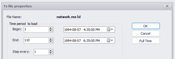
As with other selections, filtering by time when opening the file with open() is more efficient. To select time steps when opening the file, use the time parameter to specify the start and end bounds.
res = mikeio1d.open("data/network.res1d", time=('1994-08-07 16:35:00', '1994-08-07 16:38'))res.read()
WaterLevel:1
WaterLevel:2
WaterLevel:3
WaterLevel:4
WaterLevel:5
WaterLevel:6
WaterLevel:7
WaterLevel:8
WaterLevel:9
WaterLevel:10
...
Discharge:99l1:22.2508
WaterLevel:9l1:0
WaterLevel:9l1:10
Discharge:9l1:5
WaterLevel:Weir:119w1:0
WaterLevel:Weir:119w1:1
Discharge:Weir:119w1:0.5
WaterLevel:Pump:115p1:0
WaterLevel:Pump:115p1:82.4281
Discharge:Pump:115p1:41.214
1994-08-07 16:35:00.000
195.052994
195.821503
195.8815
193.604996
193.615005
193.625000
193.675003
193.764999
193.774994
193.804993
...
0.000002
193.774994
193.764999
0.000031
193.550003
188.479996
0.0
193.304993
195.005005
0.0
1994-08-07 16:36:01.870
195.052994
195.821701
195.8815
193.604996
193.615005
193.625320
193.675110
193.765060
193.775116
193.804993
...
0.000002
193.775070
193.765060
0.000031
193.550003
188.479996
0.0
193.306061
195.005005
0.0
1994-08-07 16:37:07.560
195.052994
195.821640
195.8815
193.604996
193.615005
193.625671
193.675369
193.765106
193.775513
193.804993
...
0.000002
193.775391
193.765106
0.000033
193.550034
188.479996
0.0
193.307144
195.005005
0.0
3 rows × 495 columns
To select every nth time step, you can use the step_every parameter:
res = mikeio1d.open("data/network.res1d", step_every=5)res.read().head()
WaterLevel:1
WaterLevel:2
WaterLevel:3
WaterLevel:4
WaterLevel:5
WaterLevel:6
WaterLevel:7
WaterLevel:8
WaterLevel:9
WaterLevel:10
...
Discharge:99l1:22.2508
WaterLevel:9l1:0
WaterLevel:9l1:10
Discharge:9l1:5
WaterLevel:Weir:119w1:0
WaterLevel:Weir:119w1:1
Discharge:Weir:119w1:0.5
WaterLevel:Pump:115p1:0
WaterLevel:Pump:115p1:82.4281
Discharge:Pump:115p1:41.214
1994-08-07 16:35:00.000
195.052994
195.821503
195.8815
193.604996
193.615005
193.625000
193.675003
193.764999
193.774994
193.804993
...
0.000002
193.774994
193.764999
0.000031
193.550003
188.479996
0.0
193.304993
195.005005
0.0
1994-08-07 16:40:55.828
195.052994
195.821503
195.8815
193.604996
193.615005
193.626877
193.676117
193.765457
193.776596
193.805038
...
0.000002
193.776382
193.765457
0.000042
193.550110
188.479996
0.0
193.310852
195.005005
0.0
1994-08-07 16:45:55.828
195.052994
195.821503
195.8815
193.604996
193.615128
193.628540
193.676895
193.766235
193.777557
193.805786
...
0.000003
193.777252
193.766235
0.000053
193.550125
188.479996
0.0
193.315674
195.005005
0.0
1994-08-07 16:51:29.529
195.099609
195.821655
195.8815
193.605225
193.624008
193.648056
193.678299
193.774384
193.795883
193.829300
...
0.000717
193.794693
193.774384
0.000513
193.550461
188.479996
0.0
193.321274
195.005005
0.0
1994-08-07 16:58:12.888
195.088943
195.821503
195.8815
193.607758
193.634552
193.672958
193.706161
193.829422
193.852097
193.869766
...
0.001972
193.846848
193.829422
0.005163
193.555649
188.479996
0.0
193.353027
195.005005
0.0
5 rows × 495 columns
Notice that these options are similar to when loading network result files in MIKE+:
Loading network results in MIKE+
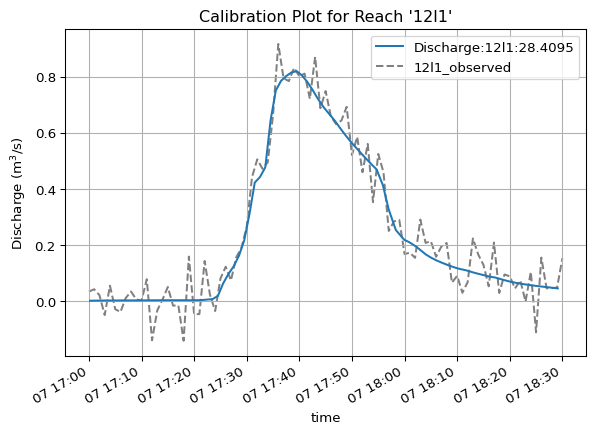
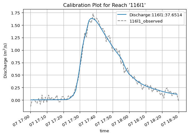
19.5 Practical Example
Imagine you’re calibrating a MIKE+ model. There’s two specific points in the network where you have observed flow data. You also have a list of calibration event time stamps you deem relevant. Let’s use Python to automate generating some plots that could be useful during the calibration process.
First, make a list of the reach IDs where the flow meters are.
calibration_points = ["12l1", "116l1"]
Next let’s define the event start and stop times.
calibration_events = [ ("1994-08-07 17:00", "1994-08-07 18:30"),# here we could add another event, but for this example we only use one]
Load the flow meter data from csv.
import pandas as pddf_obs = pd.read_csv("data/flow_meter_data.csv", index_col=0, parse_dates=True)df_obs.head()
116l1_observed
12l1_observed
time
1994-08-07 16:35:00
-0.014113
-0.095583
1994-08-07 16:36:00
0.043355
-0.058748
1994-08-07 16:37:00
-0.129244
0.040089
1994-08-07 16:38:00
-0.052462
0.068110
1994-08-07 16:39:00
-0.051976
-0.024882
Now let’s create plots for each calibration point:
for event in calibration_events: event_start = event[0] # event start time event_end = event[1] # event end time res = mikeio1d.open("data/network.res1d", time=(event_start, event_end)) df_obs_event = df_obs.loc[event_start : event_end]for reach in calibration_points: ax = res.reaches[reach].Discharge.plot() df_obs_event[f"{reach}_observed"].plot(ax=ax, color='grey', linestyle="--", zorder=-1) ax.legend() ax.grid() ax.set_title(f"Calibration Plot for Reach '{reach}'")# optional: save the figure to a PNG file using standard Matplotlib functionality