import mikeio1d

res = mikeio1d.open("data/network.res1d")
res<mikeio1d.Res1D>This section guides you through loading network results (e.g., from res1d files) into Pandas DataFrames. The approach is similar to that used with MIKE IO, allowing you to apply your DataFrame knowledge to network results.
The general workflow for network results in MIKE IO 1D is as follows:
Res1D object.Res1D object to select specific locations, quantities, or time steps.This workflow is quite similar to the one you learned in Module 2 for handling dfs0 files with MIKE IO. The core idea of opening a file, accessing data, and then often converting to a DataFrame remains consistent.
The Res1D object is central to interacting with 1D network result files. It acts as the primary container for your simulation data, analogous to MIKE IO’s Dataset object for other DHI file types.
To start, you open your result file using mikeio1d.open():
import mikeio1d
res = mikeio1d.open("data/network.res1d")
res<mikeio1d.Res1D>MIKE IO uses read() to create a Dataset, whereas MIKE IO 1D uses open() to create a Res1D object.
Get an overview of key meta data with info().
res.info()Start time: 1994-08-07 16:35:00
End time: 1994-08-07 18:35:00
# Timesteps: 110
# Catchments: 0
# Nodes: 119
# Reaches: 118
# Globals: 0
0 - Water level (m)
1 - Discharge (m^3/s)Notice the this produces similar information to that of a MIKE IO Dataset:
Like dfs0 files, all results within a Res1D object share a common time axis.
The read() method is the primary way to convert data from a Res1D object (or its subsets) into a Pandas DataFrame. This is a versatile method that can be called at various levels.
You can convert the entire content of the Res1D object into a single DataFrame. Each quantity at a specific location becomes a column in the DataFrame.
df = res.read()
df.head()| WaterLevel:1 | WaterLevel:2 | WaterLevel:3 | WaterLevel:4 | WaterLevel:5 | WaterLevel:6 | WaterLevel:7 | WaterLevel:8 | WaterLevel:9 | WaterLevel:10 | ... | Discharge:99l1:22.2508 | WaterLevel:9l1:0 | WaterLevel:9l1:10 | Discharge:9l1:5 | WaterLevel:Weir:119w1:0 | WaterLevel:Weir:119w1:1 | Discharge:Weir:119w1:0.5 | WaterLevel:Pump:115p1:0 | WaterLevel:Pump:115p1:82.4281 | Discharge:Pump:115p1:41.214 | |
|---|---|---|---|---|---|---|---|---|---|---|---|---|---|---|---|---|---|---|---|---|---|
| 1994-08-07 16:35:00.000 | 195.052994 | 195.821503 | 195.8815 | 193.604996 | 193.615005 | 193.625000 | 193.675003 | 193.764999 | 193.774994 | 193.804993 | ... | 0.000002 | 193.774994 | 193.764999 | 0.000031 | 193.550003 | 188.479996 | 0.0 | 193.304993 | 195.005005 | 0.0 |
| 1994-08-07 16:36:01.870 | 195.052994 | 195.821701 | 195.8815 | 193.604996 | 193.615005 | 193.625320 | 193.675110 | 193.765060 | 193.775116 | 193.804993 | ... | 0.000002 | 193.775070 | 193.765060 | 0.000031 | 193.550003 | 188.479996 | 0.0 | 193.306061 | 195.005005 | 0.0 |
| 1994-08-07 16:37:07.560 | 195.052994 | 195.821640 | 195.8815 | 193.604996 | 193.615005 | 193.625671 | 193.675369 | 193.765106 | 193.775513 | 193.804993 | ... | 0.000002 | 193.775391 | 193.765106 | 0.000033 | 193.550034 | 188.479996 | 0.0 | 193.307144 | 195.005005 | 0.0 |
| 1994-08-07 16:38:55.828 | 195.052994 | 195.821503 | 195.8815 | 193.604996 | 193.615005 | 193.626236 | 193.675751 | 193.765228 | 193.776077 | 193.804993 | ... | 0.000002 | 193.775894 | 193.765228 | 0.000037 | 193.550079 | 188.479996 | 0.0 | 193.308884 | 195.005005 | 0.0 |
| 1994-08-07 16:39:55.828 | 195.052994 | 195.821503 | 195.8815 | 193.604996 | 193.615005 | 193.626556 | 193.675949 | 193.765335 | 193.776352 | 193.804993 | ... | 0.000002 | 193.776154 | 193.765335 | 0.000039 | 193.550095 | 188.479996 | 0.0 | 193.309860 | 195.005005 | 0.0 |
5 rows × 495 columns
The DataFrame above includes all reaches and nodes, which results in many columns. To create more manageable DataFrames, call read() on data subsets (e.g., by location or quantity).
For example, all results for the location group reaches:
df_reaches = res.reaches.read()
df_reaches.head()| WaterLevel:100l1:0 | WaterLevel:100l1:47.6827 | WaterLevel:101l1:0 | WaterLevel:101l1:66.4361 | WaterLevel:102l1:0 | WaterLevel:102l1:10.9366 | WaterLevel:103l1:0 | WaterLevel:103l1:26.0653 | WaterLevel:104l1:0 | WaterLevel:104l1:34.4131 | ... | Discharge:93l1:24.5832 | Discharge:94l1:21.2852 | Discharge:95l1:21.9487 | Discharge:96l1:14.9257 | Discharge:97l1:5.71207 | Discharge:98l1:8.00489 | Discharge:99l1:22.2508 | Discharge:9l1:5 | Discharge:Weir:119w1:0.5 | Discharge:Pump:115p1:41.214 | |
|---|---|---|---|---|---|---|---|---|---|---|---|---|---|---|---|---|---|---|---|---|---|
| 1994-08-07 16:35:00.000 | 195.441498 | 194.661499 | 195.931503 | 195.441498 | 193.550003 | 193.550003 | 195.801498 | 195.701508 | 197.072006 | 196.962006 | ... | 0.000004 | 0.000003 | 0.000001 | 0.000005 | 0.000013 | 0.000003 | 0.000002 | 0.000031 | 0.0 | 0.0 |
| 1994-08-07 16:36:01.870 | 195.441498 | 194.661621 | 195.931503 | 195.441605 | 193.550140 | 193.550064 | 195.801498 | 195.703171 | 197.072006 | 196.962051 | ... | 0.000004 | 0.000003 | 0.000001 | 0.000005 | 0.000010 | 0.000003 | 0.000002 | 0.000031 | 0.0 | 0.0 |
| 1994-08-07 16:37:07.560 | 195.441498 | 194.661728 | 195.931503 | 195.441620 | 193.550232 | 193.550156 | 195.801498 | 195.703400 | 197.072006 | 196.962082 | ... | 0.000004 | 0.000003 | 0.000001 | 0.000005 | 0.000010 | 0.000003 | 0.000002 | 0.000033 | 0.0 | 0.0 |
| 1994-08-07 16:38:55.828 | 195.441498 | 194.661804 | 195.931503 | 195.441605 | 193.550369 | 193.550308 | 195.801498 | 195.703690 | 197.072006 | 196.962112 | ... | 0.000004 | 0.000003 | 0.000001 | 0.000005 | 0.000009 | 0.000003 | 0.000002 | 0.000037 | 0.0 | 0.0 |
| 1994-08-07 16:39:55.828 | 195.441498 | 194.661972 | 195.931503 | 195.441605 | 193.550430 | 193.550369 | 195.801498 | 195.703827 | 197.072006 | 196.962128 | ... | 0.000004 | 0.000003 | 0.000001 | 0.000005 | 0.000009 | 0.000003 | 0.000002 | 0.000039 | 0.0 | 0.0 |
5 rows × 376 columns
Or results for a reach named 100l1:
df_reach_100l1 = res.reaches["100l1"].read()
df_reach_100l1.head()| WaterLevel:100l1:0 | WaterLevel:100l1:47.6827 | Discharge:100l1:23.8414 | |
|---|---|---|---|
| 1994-08-07 16:35:00.000 | 195.441498 | 194.661499 | 0.000006 |
| 1994-08-07 16:36:01.870 | 195.441498 | 194.661621 | 0.000006 |
| 1994-08-07 16:37:07.560 | 195.441498 | 194.661728 | 0.000006 |
| 1994-08-07 16:38:55.828 | 195.441498 | 194.661804 | 0.000006 |
| 1994-08-07 16:39:55.828 | 195.441498 | 194.661972 | 0.000006 |
Or just the Discharge quantity of the previous reach.
df_reach_100l1_q = res.reaches["100l1"].Discharge.read()
df_reach_100l1_q.head()| Discharge:100l1:23.8414 | |
|---|---|
| 1994-08-07 16:35:00.000 | 0.000006 |
| 1994-08-07 16:36:01.870 | 0.000006 |
| 1994-08-07 16:37:07.560 | 0.000006 |
| 1994-08-07 16:38:55.828 | 0.000006 |
| 1994-08-07 16:39:55.828 | 0.000006 |
In the coming sections, we will cover how to explore the network structure of Res1D and select data. For now, just know that it’s possible to call read() from various sub-objects of Res1D to obtain a DataFrame.
Once you have your network data in a Pandas DataFrame using .read(), you can apply all the powerful analysis, manipulation, and visualization techniques you learned in Module 1 and Module 2.
For convenience, a plot() method is available anywhere that read() can be called. This allows for quick visualization of the data.
res.reaches["100l1"].Discharge.plot()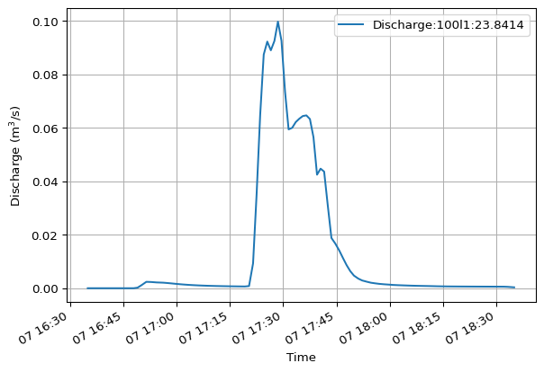
Similarly, wherever read() is available, you can export data to other common formats. For example:
res.reaches["100l1"].Discharge.to_dfs0("discharge_of_interest.dfs0")res.reaches["100l1"].Discharge.to_csv("discharge_of_interest.csv")Let’s combine some of these concepts to accomplish the following objectives:
First, open the result file.
import mikeio1d

res = mikeio1d.open("data/network.res1d")
Then, get our node water levels and reach discharges into DataFrames.
df_nodes_wl = res.nodes.WaterLevel.read()
df_reaches_q = res.reaches.Discharge.read()
Use describe() on each DataFrame, just like from previous modules.
wl_stats = df_nodes_wl.describe().T
wl_stats.head()| count | mean | std | min | 25% | 50% | 75% | max | |
|---|---|---|---|---|---|---|---|---|
| WaterLevel:1 | 110.0 | 195.198898 | 0.159523 | 195.052994 | 195.090881 | 195.131989 | 195.258179 | 195.669006 |
| WaterLevel:2 | 110.0 | 195.822342 | 0.000657 | 195.821503 | 195.821503 | 195.822784 | 195.822937 | 195.822968 |
| WaterLevel:3 | 110.0 | 195.881470 | 0.000000 | 195.881500 | 195.881500 | 195.881500 | 195.881500 | 195.881500 |
| WaterLevel:4 | 110.0 | 193.947418 | 0.348278 | 193.604996 | 193.614719 | 193.891739 | 194.173325 | 194.661331 |
| WaterLevel:5 | 110.0 | 194.010544 | 0.379473 | 193.615005 | 193.659035 | 193.940742 | 194.260757 | 194.793060 |
q_stats = df_reaches_q.describe().T
q_stats.head()| count | mean | std | min | 25% | 50% | 75% | max | |
|---|---|---|---|---|---|---|---|---|
| Discharge:100l1:23.8414 | 110.0 | 0.014078 | 0.026875 | 0.000006 | 0.000636 | 0.001032 | 0.005988 | 0.099751 |
| Discharge:101l1:33.218 | 110.0 | -0.000034 | 0.005649 | -0.022655 | 0.000004 | 0.000005 | 0.000022 | 0.019202 |
| Discharge:102l1:5.46832 | 110.0 | 0.069058 | 0.100331 | -0.011316 | 0.003062 | 0.017987 | 0.096062 | 0.326383 |
| Discharge:103l1:13.0327 | 110.0 | -0.000011 | 0.001084 | -0.006748 | 0.000002 | 0.000017 | 0.000337 | 0.001056 |
| Discharge:104l1:17.2065 | 110.0 | 0.000005 | 0.000002 | 0.000003 | 0.000005 | 0.000005 | 0.000005 | 0.000025 |
From here we might want to use existing Pandas functionality to export our data for reporting purposes:
wl_stats.to_excel("node_water_levels.xlsx")
q_stats.to_excel("reaches_discharges.xlsx")You need to install a Python package like openpyxl to use Pandas’ to_excel() method.