Now that you’ve prepared your Observation and ModelResult data, the next crucial step is to bring them together for direct comparison. ModelSkill makes this easy with ms.match() which creates a Comparer object. For situations where you need to assess performance across multiple locations or aggregate results, you can group several Comparer objects into a ComparerCollection.
This section uses Observation and ModelResult objects prepared as in previous examples.
Show setup code for Observation and ModelResult objects
# Source datasetsds_obs_source = mikeio.read("data/flow_meter_data.dfs0")ds_model_source = mikeio.read("data/model_results.dfs0")# Observation for 116l1obs_116l1 = ms.PointObservation( data=ds_obs_source, item="116l1_observed", name="116l1"# Unique name for this observation point)# Observation for 12l1obs_12l1 = ms.PointObservation( data=ds_obs_source, item="12l1_observed", name="12l1"# Unique name for this observation point)# Model Result for 116l1 from MIKE+mod_116l1 = ms.PointModelResult( data=ds_model_source, item="reach:Discharge:116l1:37.651", name="MIKE+"# Name of the model simulation)# Model Result for 12l1 from MIKE+mod_12l1 = ms.PointModelResult( data=ds_model_source, item="reach:Discharge:12l1:28.410", name="MIKE+"# Name of the model simulation (same as above))
Comparer
Use ms.match() to create a Comparer object. A Comparer is designed to match one Observation with one ModelResult. For point data, match() intelligently interpolates model results to observation timestamps, ensuring a direct, like-for-like comparison.
Let’s match our previously defined obs_116l1 with mod_116l1:
The Comparer now conveniently holds your matched data, interpolated and aligned, ready for detailed analysis and visualization. You can convert this to a Pandas DataFrame to inspect the aligned data. Notice how the DataFrame contains raw observation values and model values interpolated to the exact observation times.
It’s crucial that the Observation and ModelResult objects passed to ms.match() represent the same physical location and variable. ModelSkill relies on you to provide these correctly paired inputs.
Handling Gaps in Model Data During Matching
When matching, ModelSkill interpolates model results to observation times. If your model data has significant time gaps, you might not want to interpolate across very large intervals. For example, this is often the case with LTS simulations. The max_model_gap parameter in ms.match() controls this. It specifies the maximum gap (in seconds) in the model data over which to interpolate. If a gap is larger, the corresponding observation points will not have a matched model value.
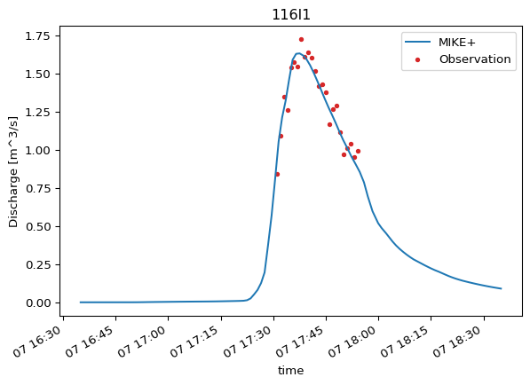
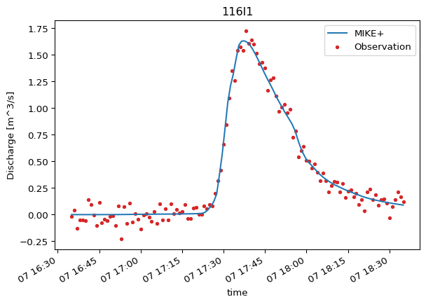
A Comparer object is your gateway to generating insightful plots and calculating a range of skill scores. Plotting and skill assessment are detailed later in this module, but here’s a quick preview:
comparer_116l1.plot.timeseries()
comparer_116l1.skill()
n
bias
rmse
urmse
mae
cc
si
r2
observation
116l1
121
0.003229
0.068114
0.068037
0.054517
0.991234
0.172594
0.982405
Filtering Matched Data
After matching, you might want to further filter the Comparer data before calculating skill scores. For example, you might want to exclude periods of low flow or focus only on specific events. The .query() method allows you to apply conditions, similar to Pandas. It returns a new Comparer object with the filtered data.
ModelSkill offers more filtering options not covered here — see the documentation for details.
ComparerCollection
Often, you’ll want to evaluate your model against multiple observation points simultaneously or assess its overall performance across different locations. For this, ModelSkill provides the ComparerCollection, which groups multiple Comparer objects.
Comparing models against other models
A ComparerCollection can also be used to compare multiple different models against the same set of observations. That use case is not covered in this module. Refer to ModelSkill’s documentation for details on this powerful feature.
First, let’s create another Comparer for our second observation point, obs_12l1, and its corresponding model result, mod_12l1 (which comes from the same MIKE+ simulation).
The ComparerCollection (cc) now manages both comparisons. This allows for powerful aggregate views. For instance, it provides skill assessment for each individual observation:
cc.skill()
n
bias
rmse
urmse
mae
cc
si
r2
observation
116l1
121
0.003229
0.068114
0.068037
0.054517
0.991234
0.172594
0.982405
12l1
121
-0.004083
0.063414
0.063282
0.049679
0.971574
0.305942
0.942928
More importantly, it enables aggregate views of model performance, such as overall skill scores that consider all included comparisons:
cc.mean_skill()
n
bias
rmse
urmse
mae
cc
si
r2
model
MIKE+
242
-0.000427
0.065764
0.06566
0.052098
0.981404
0.239268
0.962667
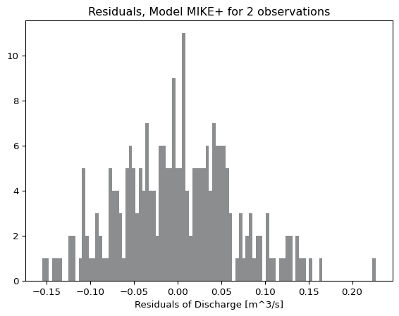
And aggregate plots, like a histogram of residual errors across all matched observation points:
cc.plot.residual_hist()
You can inspect the collection’s properties to see which observations and models are included:
Unique observation names within the collection:
cc.obs_names
['116l1', '12l1']
Unique model names. Since both mod_116l1 and mod_12l1 were created with name="MIKE+", “MIKE+” appears only once, signifying they are from the same model run.
cc.mod_names
['MIKE+']
You can also select an individual Comparer from the collection by its observation name, allowing you to focus on a specific comparison: