This section guides you through loading time series data from dfs0 files into Pandas DataFrames. This approach allows you to leverage your existing Pandas skills, learned in Module 1, for powerful time series analysis and manipulation.
10.1 Workflow
The general workflow for working with dfs0 data is as follows:
Read dfs0 file into Dataset
Subset Dataset for specific items and times (optional)
Convert Dataset (or DataArray) to DataFrame
Perform some additional analysis via the DataFrame
10.2 Datasets
The primary function for reading MIKE IO files is mikeio.read(). It returns a Dataset object, which is a container for one or more DataArray objects (e.g. a specific time series).
Reading a dfs0 file into a Dataset is as simple as calling the read() method with the dfs0 file path as the argument:
Notice the representation of the Dataset object shows information about:
Total number of time steps
Timestamps for first and last time step
All the items (i.e. DataArrays) available
Read() loads entire dfs0 into memory by default
By default, mikeio.read() loads the entire dfs0 file into memory. This is fine for smaller files, but for very large dfs0 files, you might want to load only specific items or a particular time range to conserve memory and improve performance. You can do this directly with the items or time arguments in the read() function. For example, to read only the first item (index 0):
Notice the representation of the DataArray object is also informative, just like the Dataset object.
10.4 Convert to Pandas
You can convert an entire Dataset (which might contain multiple time series) into a Pandas DataFrame. Each item in the Dataset will become a column in the DataFrame.
import pandas as pdds = mikeio.read("data/sirius_idf_rainfall.dfs0")df = ds.to_dataframe()df.head()
F=20
F=10
F=5
F=2
F=1
F=0.5
F=0.2
F=0.1
F=0.05
2019-01-01 00:00:00
0.00
0.000000
0.0
0.0
0.000000
0.000000
0.000000
0.000000
0.0
2019-01-01 06:00:00
0.15
0.283333
0.4
0.4
0.466667
0.683333
0.966667
1.316667
1.4
2019-01-01 07:00:00
0.20
0.400000
0.6
0.6
0.800000
1.100000
1.600000
2.200000
2.3
2019-01-01 08:00:00
0.30
0.600000
0.7
0.8
0.900000
1.400000
2.000000
2.800000
3.1
2019-01-01 09:00:00
0.30
0.600000
0.9
1.0
1.200000
1.800000
2.600000
3.600000
4.0
Similarly, a single DataArray can be converted to a Pandas DataFrame (which will have one data column).
da = ds[" F=20"]df_T20 = da.to_dataframe()df_T20.head()
F=20
2019-01-01 00:00:00
0.00
2019-01-01 06:00:00
0.15
2019-01-01 07:00:00
0.20
2019-01-01 08:00:00
0.30
2019-01-01 09:00:00
0.30
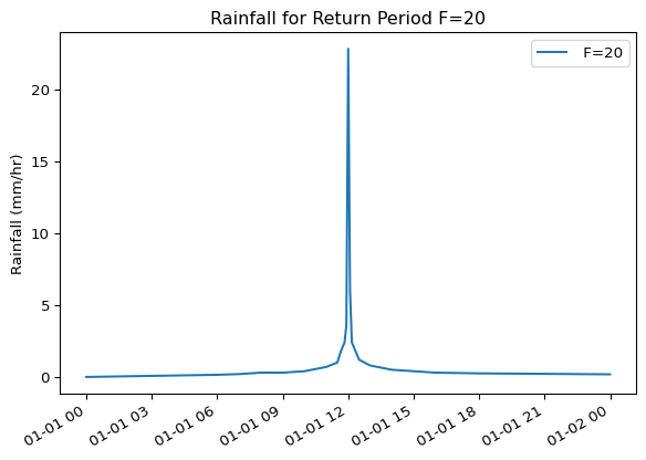
Once your data is in a DataFrame, you can use all of Pandas’ powerful methods. For instance, you can easily plot a time series:
df_T20.plot( title="Rainfall for Return Period F=20", ylabel="Rainfall (mm/hr)")
Or get some descriptive statistics:
df.describe().T
count
mean
std
min
25%
50%
75%
max
F=20
22.0
2.158333
4.824954
0.0
0.300
0.60
1.80
22.799999
F=10
22.0
4.039394
9.101874
0.0
0.525
1.10
3.00
43.200001
F=5
22.0
5.890909
13.389296
0.0
0.725
1.60
4.65
63.599998
F=2
22.0
9.408333
17.422466
0.0
0.825
2.00
8.40
75.599998
F=1
22.0
12.641667
25.616199
0.0
0.950
2.40
9.75
114.000000
F=0.5
22.0
15.833333
30.442241
0.0
1.425
3.40
13.50
134.399994
F=0.2
22.0
22.475000
36.939988
0.0
2.075
5.30
23.40
151.199997
F=0.1
22.0
27.500758
39.726610
0.0
2.900
7.60
34.05
153.600006
F=0.05
22.0
30.627272
42.803784
0.0
3.200
8.65
39.75
158.399994
Learning Python’s scientific ecosystem pays off…
Notice that using a common structure for data (e.g. DataFrame) unlocks familiar analyses independent of the original data source file format (e.g. dfs0, csv). This is an example of why converting data into a format compatible with the scientific Python ecosystem is useful.