Dfs3

A dfs3 file stores gridded data with three spatial dimensions. Like dfs2, values are ‘element based’, i.e. defined in the centre of each grid cell. The layers are ordered from the bottom up, so the last layer is the top one.

import mikeio

ds = mikeio.read("../data/dissolved_oxygen.dfs3")
ds
<mikeio.Dataset>
title: Area from:  f00dek125_
dims: (time:1, z:17, y:112, x:91)
time: 2001-12-28 00:00:00 (time-invariant)
geometry: Grid3D(nz=17, ny=112, nx=91)
items:
  0:  Diss. oxygen (mg/l) <Concentration 3> (mg per liter)

Grid3D

The spatial information is available in the geometry attribute (accessible from Dfs3, Dataset, and DataArray), which for a dfs3 file is a Grid3D geometry.

ds.geometry
<mikeio.Grid3D>
x: [0, 150, ..., 1.35e+04] (nx=91, dx=150)
y: [0, 150, ..., 1.665e+04] (ny=112, dy=150)
z: [0, 1, ..., 16] (nz=17, dz=1)
origin: (5.864e+05, 6.143e+06), orientation: 17.000
projection: PROJCS["UTM-32",GEOGCS["Unused",DATUM["UTM Projections",SPHEROID["WGS 1984",6378137,298.257223563]],PRIMEM["Greenwich",0],UNIT["Degree",0.0174532925199433]],PROJECTION["Transverse_Mercator"],PARAMETER["False_Easting",500000],PARAMETER["False_Northing",0],PARAMETER["Central_Meridian",9],PARAMETER["Scale_Factor",0.9996],PARAMETER["Latitude_Of_Origin",0],UNIT["Meter",1]]

The horizontal axes behave as they do for dfs2. The vertical one is described by z, nz and dz, and is numbered from the bottom up, so the last layer is the top one. See the API reference for the full set of properties and methods.

A dfs3 file with only one layer is read as a Grid2D rather than a Grid3D, since there is no vertical dimension left to describe.

Selecting layers while reading

A dfs3 file covering many layers and time steps can be large, and often only one layer is of interest. The layers argument selects layers during reading, so the rest of the file is never loaded into memory. It accepts "top", "bottom", or layer indices.

dst = mikeio.read("../data/dissolved_oxygen.dfs3", layers="top")
dst
<mikeio.Dataset>
title: Area from:  f00dek125_
dims: (time:1, y:112, x:91)
time: 2001-12-28 00:00:00 (time-invariant)
geometry: Grid2D (ny=112, nx=91)
items:
  0:  Diss. oxygen (mg/l) <Concentration 3> (mg per liter)

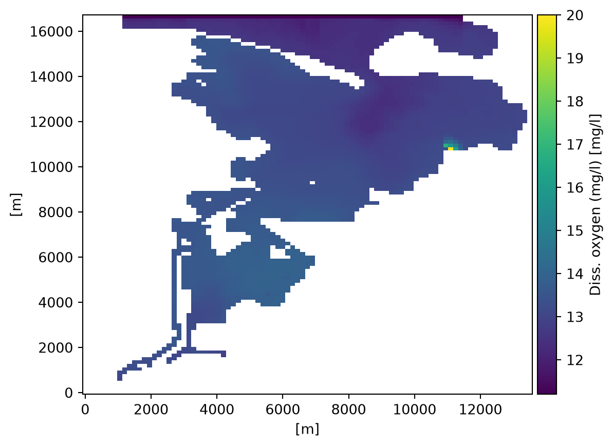
Note that the result is a two-dimensional dataset: selecting a single layer drops the z dimension and the geometry becomes a Grid2D, which can be plotted and written to a dfs2 file.

dst[0].plot();

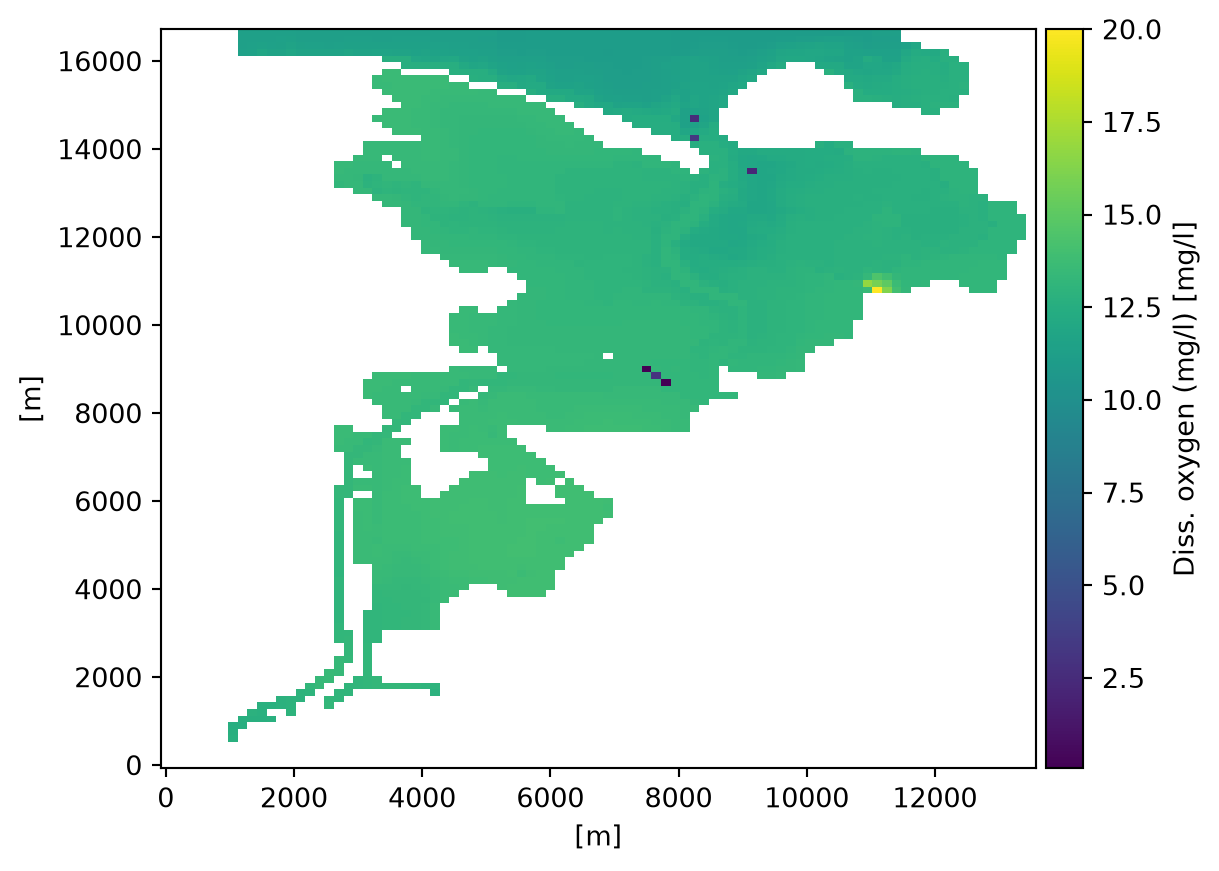
Reading the bottom layer instead shows a different picture, since oxygen is consumed near the bed.

dsb = mikeio.read("../data/dissolved_oxygen.dfs3", layers="bottom")
dsb[0].plot();

Note that "top" and "bottom" are not fixed layer numbers. A dfs3 covering a domain with varying depth has cells that hold no data, and the two keywords select the highest and lowest cell that does hold data in each column. The layer they come from therefore differs from one horizontal position to the next, which is why layers="bottom" is not the same as layers=[0]:

import numpy as np

nz = ds.geometry.nz
bottom = mikeio.read("../data/dissolved_oxygen.dfs3", layers="bottom")[0].to_numpy()
layer0 = mikeio.read("../data/dissolved_oxygen.dfs3", layers=[0])[0].to_numpy()
top = mikeio.read("../data/dissolved_oxygen.dfs3", layers="top")[0].to_numpy()
last = mikeio.read("../data/dissolved_oxygen.dfs3", layers=[nz - 1])[0].to_numpy()

np.allclose(bottom, layer0, equal_nan=True), np.allclose(top, last, equal_nan=True)
(False, True)

The top layer happens to coincide with the last one in this file, because its surface layer is wet everywhere.

Selecting layers after reading

If the whole file is already in memory, use isel along the z dimension. Layer -1 is the top layer and 0 the bottom one.

do = ds["Diss. oxygen (mg/l)"]
do.isel(z=-1)
<mikeio.DataArray>
name: Diss. oxygen (mg/l)
dims: (time:1, y:112, x:91)
time: 2001-12-28 00:00:00 (time-invariant)
geometry: Grid2D (ny=112, nx=91)

Selecting along x instead gives a vertical slice through the domain. Note that spatial selection on a Grid3D is by index rather than by coordinate: unlike dfs2, sel(x=..., y=...) is not available for three-dimensional grids, and isel takes one dimension at a time.

do.isel(x=56)
<mikeio.DataArray>
name: Diss. oxygen (mg/l)
dims: (time:1, y:17, x:112)
time: 2001-12-28 00:00:00 (time-invariant)
geometry: Grid2D (ny=17, nx=112)

Local coordinates

Local coordinates (“NON-UTM”) follow a different convention to projected ones: the origin sits at the bottom-left corner of the grid rather than at the centre of the first element. This applies to the x and y coordinates.
import numpy as np

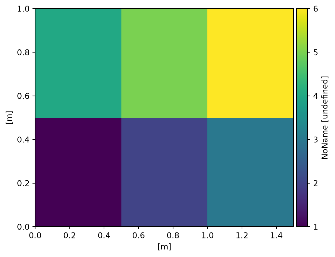
data = np.array([[[1.0, 2, 3], [4, 5, 6]], [[7, 8, 9], [10, 11, 12]]])
da = mikeio.DataArray(
    data,
    geometry=mikeio.Grid3D(nx=3, ny=2, nz=2, dx=0.5, dy=0.5, dz=1, projection="NON-UTM"),
)
da.geometry
<mikeio.Grid3D>
x: [0.25, 0.75, 1.25] (nx=3, dx=0.5)
y: [0.25, 0.75] (ny=2, dy=0.5)
z: [0, 1] (nz=2, dz=1)
origin: (0, 0), orientation: 0.000
projection: NON-UTM

The origin is (0, 0), and the first cell centre is therefore half a cell width away from it:

da.geometry.x
array([0.25, 0.75, 1.25])
da.isel(z=0).plot();

Converting to xarray

A dfs3 DataArray converts to an xarray DataArray, which is convenient for writing NetCDF or for combining with other gridded data.

da.to_xarray()
<xarray.DataArray 'NoName' (z: 2, y: 2, x: 3)> Size: 96B
array([[[ 1.,  2.,  3.],
        [ 4.,  5.,  6.]],

       [[ 7.,  8.,  9.],
        [10., 11., 12.]]])
Coordinates:
  * z        (z) float64 16B 0.0 1.0
  * y        (y) float64 16B 0.25 0.75
  * x        (x) float64 24B 0.25 0.75 1.25
Attributes:
    name:     NoName
    units:    undefined
    eumType:  999
    eumUnit:  0