Generic dfs processing

Tools and methods that applies to any type of dfs files.

The generic tools are useful for common data processing tasks, where detailed configuration is not necessary.

mikeio.generic: methods that read any dfs file and outputs a new dfs file of the same type

• concat: Concatenates files along the time axis

• scale: Apply scaling to any dfs file

• sum: Sum two dfs files

• diff: Calculate difference between two dfs files

• extract: Extract timesteps and/or items to a new dfs file

• time-avg: Create a temporally averaged dfs file

• quantile: Create temporal quantiles of dfs file

The generic methods works on larger-than-memory files as they process one time step at a time. This can however make them in-efficient for dfs0 processing!

See Generic in MIKE IO Documentation

import matplotlib.pyplot as plt

import mikeio
import mikeio.generic

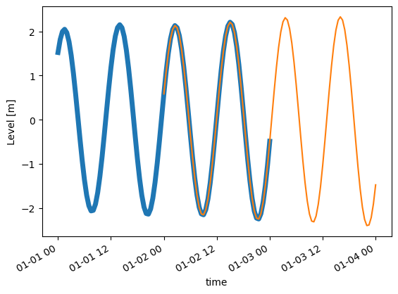
Concatenation

Take a look at these two files with overlapping timesteps.

t1 = mikeio.read("data/tide1.dfs1")
t1

<mikeio.Dataset>
dims: (time:97, x:10)
time: 2019-01-01 00:00:00 - 2019-01-03 00:00:00 (97 records)
geometry: Grid1D (n=10, dx=0.06667)
items:
  0:  Level <Water Level> (meter)

t2 = mikeio.read("data/tide2.dfs1")
t2

<mikeio.Dataset>
dims: (time:97, x:10)
time: 2019-01-02 00:00:00 - 2019-01-04 00:00:00 (97 records)
geometry: Grid1D (n=10, dx=0.06667)
items:
  0:  Level <Water Level> (meter)

Plot one of the points along the line.

ax = t1[0].isel(x=1).plot(lw=5)
t2[0].isel(x=1).plot(ax=ax);

mikeio.generic.concat(infilenames=["data/tide1.dfs1",
                                   "data/tide2.dfs1"],
                      outfilename="concat.dfs1")

  0%|          | 0/2 [00:00<?, ?it/s]

100%|██████████| 2/2 [00:00<00:00, 667.14it/s]

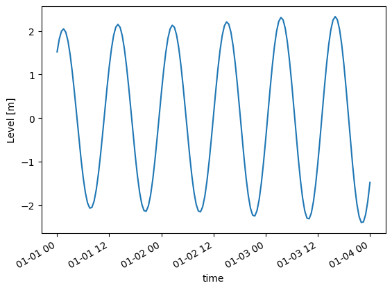
c = mikeio.read("concat.dfs1")
c

<mikeio.Dataset>
dims: (time:145, x:10)
time: 2019-01-01 00:00:00 - 2019-01-04 00:00:00 (145 records)
geometry: Grid1D (n=10, dx=0.06667)
items:
  0:  Level <Water Level> (meter)

c[0].isel(x=1).plot();

Extract time steps or items

The extract() method can extract a part of a file:

• time slice by specifying start and/or end

• specific items

infile = "data/tide1.dfs1"
mikeio.generic.extract(infile, "extracted.dfs1", start='2019-01-02')

e = mikeio.read("extracted.dfs1")
e

<mikeio.Dataset>
dims: (time:49, x:10)
time: 2019-01-02 00:00:00 - 2019-01-03 00:00:00 (49 records)
geometry: Grid1D (n=10, dx=0.06667)
items:
  0:  Level <Water Level> (meter)

infile = "data/oresund_vertical_slice.dfsu"
mikeio.generic.extract(infile, "extracted.dfsu", items='Salinity', end=-2)

e = mikeio.read("extracted.dfsu")
e

<mikeio.Dataset>
dims: (time:2, element:441)
time: 1997-09-15 21:00:00 - 1997-09-16 00:00:00 (2 records)
geometry: DfsuVerticalProfileSigmaZ (441 elements, 550 nodes)
items:
  0:  Salinity <Salinity> (PSU)

Inline exercise

1. use mikeio.generic.extract to extract the data from the beginning of the file ‘data/tide2.dfs1’ until “2019-01-03”, into a new file named ‘tide_start.dfs1’

2. use mikeio.read to read the new file ‘tide_start.dfs1’ into a Dataset named ds

3. Check that the end time, ds.end_time matches what you specified above

mikeio.read("data/tide2.dfs1")

<mikeio.Dataset>
dims: (time:97, x:10)
time: 2019-01-02 00:00:00 - 2019-01-04 00:00:00 (97 records)
geometry: Grid1D (n=10, dx=0.06667)
items:
  0:  Level <Water Level> (meter)

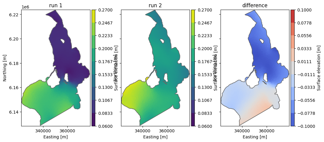
Diff

Take difference between two dfs files with same structure - e.g. to see the difference in result between two calibration runs

fn1 = "data/oresundHD_run1.dfsu"
fn2 = "data/oresundHD_run2.dfsu"
fn_diff = "oresundHD_difference.dfsu"
mikeio.generic.diff(fn1, fn2, fn_diff)

  0%|          | 0/5 [00:00<?, ?it/s]

100%|██████████| 5/5 [00:00<00:00, 2909.48it/s]

Let’s open the files and visualize the last time step of the first item (water level)

_, ax = plt.subplots(1,3, sharey=True, figsize=(12,5))
da = mikeio.read(fn1, time=-1)[0]
da.plot(vmin=0.06, vmax=0.27, ax=ax[0], title='run 1')
da = mikeio.read(fn2, time=-1)[0]
da.plot(vmin=0.06, vmax=0.27, ax=ax[1], title='run 2')
da = mikeio.read(fn_diff, time=-1)[0]
da.plot(vmin=-0.1, vmax=0.1, cmap='coolwarm', ax=ax[2], title='difference');

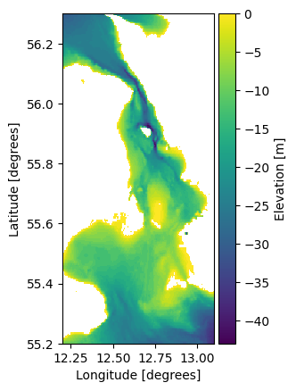
Scaling

Adding a constant e.g to adjust datum

ds = mikeio.read("data/gebco_sound.dfs2")
ds.Elevation.plot();

ds['Elevation'][0,104,131]

<mikeio.DataArray>
name: Elevation
dims: ()
time: 2020-05-15 11:04:52 (time-invariant)
geometry: GeometryPoint2D(x=12.74791669513408, y=55.63541668926675)
values: -1.0

This is the processing step.

mikeio.generic.scale("data/gebco_sound.dfs2","gebco_sound_local_datum.dfs2",offset=-2.1)

  0%|          | 0/1 [00:00<?, ?it/s]

100%|██████████| 1/1 [00:00<00:00, 987.59it/s]

ds2 = mikeio.read("gebco_sound_local_datum.dfs2")
ds.Elevation.plot();

ds2['Elevation'][0,104,131]

<mikeio.DataArray>
name: Elevation
dims: ()
time: 2020-05-15 11:04:52 (time-invariant)
geometry: GeometryPoint2D(x=12.74791669513408, y=55.63541668926675)
values: -3.0999999046325684

Spatially varying correction

import numpy as np
factor = np.ones_like(ds['Elevation'][0].to_numpy())
factor.shape

(264, 216)

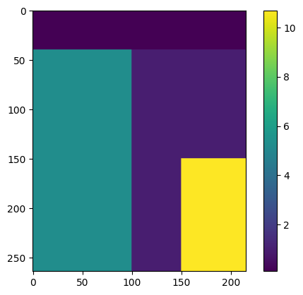
Add some spatially varying factors, exaggerated values for educational purpose.

factor[:,0:100] = 5.3
factor[0:40,] = 0.1
factor[150:,150:] = 10.7
plt.imshow(factor)
plt.colorbar();

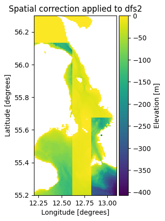
The 2d array must first be flipped upside down and then converted to a 1d vector using numpy.ndarray.flatten to match how data is stored in dfs files.

factor_ud = np.flipud(factor)
factor_vec  = factor_ud.flatten()
mikeio.generic.scale("data/gebco_sound.dfs2","gebco_sound_spatial.dfs2",factor=factor_vec)

  0%|          | 0/1 [00:00<?, ?it/s]

100%|██████████| 1/1 [00:00<00:00, 1157.05it/s]

ds3 = mikeio.read("gebco_sound_spatial.dfs2")
ds3.Elevation.plot()
plt.title("Spatial correction applied to dfs2");

Clean up

import os
os.remove("concat.dfs1")
os.remove("extracted.dfs1")
os.remove("extracted.dfsu")
os.remove("oresundHD_difference.dfsu")
os.remove("gebco_sound_local_datum.dfs2")
os.remove("gebco_sound_spatial.dfs2")

import utils

utils.sysinfo()

    System: 3.11.14 (main, Oct 10 2025, 01:03:14) [GCC 13.3.0]
    NumPy: 2.4.1
    Pandas: 2.3.3
    MIKE IO: 3.0.1
    Last modified: 2026-01-15 07:16:38.643667