Dfs1

Dfs1 has in addition to the dfs0 file a single spatial dimension.

This spatial dimension has information on the grid spacing, but do not contain enough metadata to determine their geographical position, but have a relative distance from the origo.

See Dfs1 in MIKE IO Documentation

See DFS - Reference manual

import mikeio

ds = mikeio.read("data/waterlevel_north.dfs1")
ds

<mikeio.Dataset>
dims: (time:577, x:2)
time: 1993-12-02 00:00:00 - 1993-12-14 00:00:00 (577 records)
geometry: Grid1D (n=2, dx=8800)
items:
  0:  North WL <Water Level> (meter)

ds.geometry

<mikeio.Grid1D>
x: [0, 8800] (nx=2, dx=8800)

This dfs1 file contains only two nodes (nx=2) and has a grid spacing of 8800 m.

The dataset has a single item North WL which we can access in three different ways.

1. As an attribute ds.North_WL

2. As a key in a dictionary ds["North WL"]

3. By position ds[0]

da = ds.North_WL
da

<mikeio.DataArray>
name: North WL
dims: (time:577, x:2)
time: 1993-12-02 00:00:00 - 1993-12-14 00:00:00 (577 records)
geometry: Grid1D (n=2, dx=8800)

The dataarray variable da contains all the data for the North WL item from the dfs1 file.

Visualization

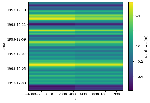
The data can be visualized with the .plot() method.

The default plot show time on the vertical axis and space on the horizontal axis since dfs1 are often used to represent horizontal variations along an open boundary.

da.plot();

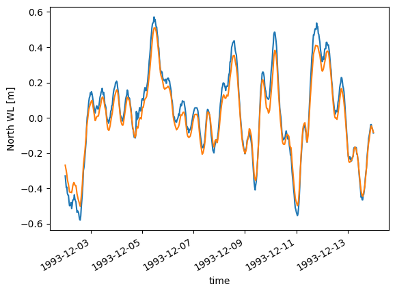
Fort this example, with only a few nodes on the spatial axis, it makes more sense to visualize the data as individual lines in a timeseries plot.

da.plot.timeseries();

Inline exercise

Are there other possible visualizations?

Spatial and temporal selection

Spatial subsetting can be done in two ways:

1. positional index using .isel() x=0..(nx-1) (or with negative indexing from the end)

2. distance along the axis using sel() x=0..8800 (pick closest node)

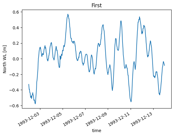
da.isel(x=0).plot(title="First");

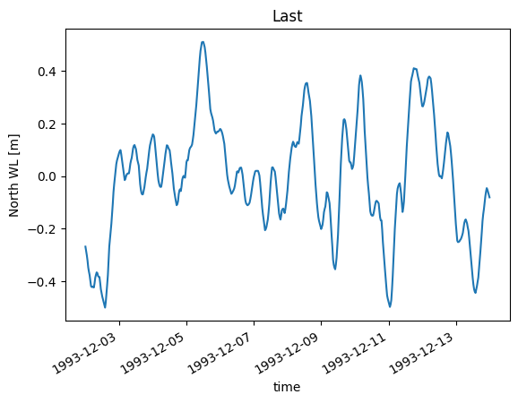
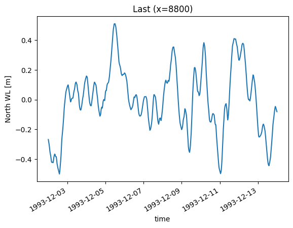
da.isel(x=-1).plot(title="Last");

da.sel(x=8800).plot(title="Last (x=8800)")

<Axes: title={'center': 'Last (x=8800)'}, xlabel='time', ylabel='North WL [m]'>

Calculated items

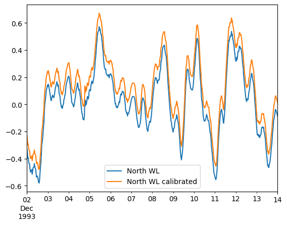
Creating a new dataarray in the dataset based on an existing dataarray is easy.

ds["North WL calibrated"] = da + 0.1 # add 0.1 m to the original data

Export to dfs0

After subsetting into a single spatial point the result no longer has any spatial dimension and has become a simple timeseries which can be saved as a dfs0 file.

ds.isel(x=0)

<mikeio.Dataset>
dims: (time:577)
time: 1993-12-02 00:00:00 - 1993-12-14 00:00:00 (577 records)
geometry: GeometryUndefined()
items:
  0:  North WL <Water Level> (meter)
  1:  North WL calibrated <Water Level> (meter)

ds.isel(x=0).geometry

GeometryUndefined()

ds.isel(x=0).to_dfs("random_0.dfs0")

mikeio.read("random_0.dfs0").plot();

Inline exercise

Export the timeseries in the last spatial element as a csv file

import utils

utils.sysinfo()

    System: 3.11.9 (main, Apr  2 2024, 15:19:53) [GCC 11.4.0]
    NumPy: 1.26.4
    Pandas: 2.2.2
    MIKE IO: 1.7.1
    Last modified: 2024-04-11 17:10:50.544541