Mesh#
See Mesh in MIKE IO Documentation
import numpy as np
import matplotlib.pyplot as plt
import mikeio
A simple mesh#
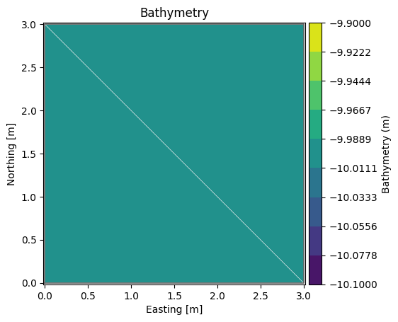
Let’s consider a simple mesh consisting of 2 triangular elements.
fn = "data/two_elements.mesh"
with open(fn, "r") as f:
    print(f.read())
100079 1000 4  UTM-31
1 0.0 0.0 -10.0 1
2 3.0 0.0 -10.0 2
3 3.0 3.0 -10.0 2
4 0.0 3.0 -10.0 1
2 3 21
1 1 2 4
2 2 3 4
msh = mikeio.open(fn)
msh
<Mesh>
number of nodes: 4
number of elements: 2
projection: UTM-31
msh.plot(show_mesh=True);
msh.geometry
Flexible Mesh Geometry: Dfsu2D
number of nodes: 4
number of elements: 2
projection: UTM-31
msh.node_coordinates
array([[  0.,   0., -10.],
       [  3.,   0., -10.],
       [  3.,   3., -10.],
       [  0.,   3., -10.]])
msh.element_table
[array([0, 1, 3], dtype=int32), array([1, 2, 3], dtype=int32)]
msh.element_coordinates
array([[  1.,   1., -10.],
       [  2.,   2., -10.]])
msh.geometry.get_element_area()
array([4.5, 4.5])
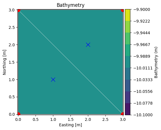
Let’s plot the node and element coordinates:
xn, yn = msh.node_coordinates[:,0], msh.node_coordinates[:,1]
xe, ye = msh.element_coordinates[:,0], msh.element_coordinates[:,1]

ax = msh.plot(show_mesh=True)
ax.plot(xn, yn, 'ro', markersize=10)
ax.plot(xe, ye, 'bx', markersize=10)
[<matplotlib.lines.Line2D at 0x7fded21a6150>]
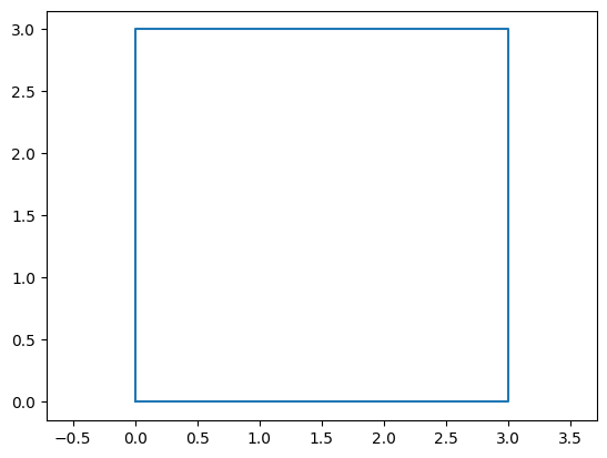
Boundary polylines#
It can sometimes be convenient to have mesh boundary as a polyline (or multiple in case of more complex meshes).
bxy = msh.geometry.boundary_polylines.exteriors[0].xy
plt.plot(bxy[:,0], bxy[:,1])
plt.axis("equal");
/opt/hostedtoolcache/Python/3.11.14/x64/lib/python3.11/site-packages/mikeio/spatial/_FM_geometry.py:802: FutureWarning: boundary_polylines is renamed to boundary_polygons
  warnings.warn(
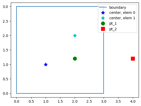
Inside domain?#
MIKE IO has a method for determining if a point (or a list of points) is inside the domain:
contains()
pt_1 = [2.0, 1.2]
msh.geometry.contains(pt_1)[0]
np.True_
# or multiple points at the same time
pt_2 = [4.0, 1.2]
pts = np.array([pt_1, pt_2])
msh.geometry.contains(pts)
array([ True, False])
plt.plot(bxy[:,0], bxy[:,1], label='boundary')
plt.plot(xe[0], ye[0], 'b*', markersize=10, label="center, elem 0")
plt.plot(xe[1], ye[1], 'c*', markersize=10, label="center, elem 1")
plt.plot(*pt_1, 'go', markersize=10, label="pt_1")
plt.plot(*pt_2, 'rs', markersize=10, label="pt_2")
plt.axis("equal")
plt.legend(loc="upper right");
Find element containing point#
MIKE IO has a method for obtaining the index of the element containing a point:
find_index()
g = msh.geometry
g.find_index(coords=pt_1)[0]
np.int64(1)
MIKE IO also has a method for obtaining a list of the n closest element centers:
find_nearest_elements()
g.find_nearest_elements(pt_1)
1
g.find_nearest_elements(pt_1, return_distances=True)
(1, 0.8)
g.find_nearest_elements(pt_1, n_nearest=2)
array([1, 0])
# for multiple points
g.find_nearest_elements(pts, return_distances=True)
(array([1, 1]), array([0.8 , 2.15406592]))
A larger mesh#
dfs = mikeio.open("data/FakeLake.dfsu")
g = dfs.geometry
g
Flexible Mesh Geometry: Dfsu2D
number of nodes: 798
number of elements: 1011
projection: PROJCS["UTM-17",GEOGCS["Unused",DATUM["UTM Projections",SPHEROID["WGS 1984",6378137,298.257223563]],PRIMEM["Greenwich",0],UNIT["Degree",0.0174532925199433]],PROJECTION["Transverse_Mercator"],PARAMETER["False_Easting",500000],PARAMETER["False_Northing",0],PARAMETER["Central_Meridian",-81],PARAMETER["Scale_Factor",0.9996],PARAMETER["Latitude_Of_Origin",0],UNIT["Meter",1]]
g.plot();
Inline Exercise#
please check if the point A: (x,y)=(-0.5, 0.0) is inside the mesh
please check if the point B: (x,y)=(-0.5, 0.4) is inside the mesh
find index of the 5 closest points to B
# insert code here
g.max_nodes_per_element
4
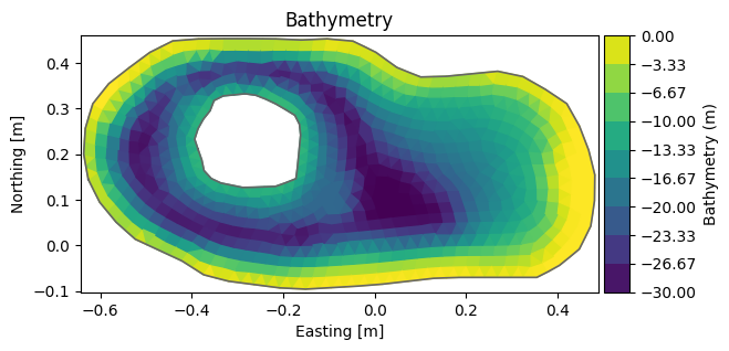
Change depth#
msh = mikeio.open("data/FakeLake.dfsu").geometry
msh.plot();
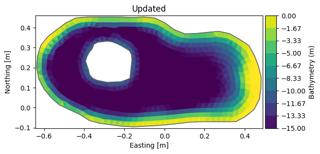
msh.node_coordinates[:,2] = np.clip(msh.node_coordinates[:,2], -15, 0) # clip depth to interval [-15,0]


msh.plot(title="No change??")
<Axes: title={'center': 'No change??'}, xlabel='Easting [m]', ylabel='Northing [m]'>

del msh.element_coordinates # remove cached element coords calculated based on original node coords)
msh.plot(title="Updated")
<Axes: title={'center': 'Updated'}, xlabel='Easting [m]', ylabel='Northing [m]'>
msh.to_mesh('Fake_lake_clip15.mesh') # save to a new file
Visualisation#
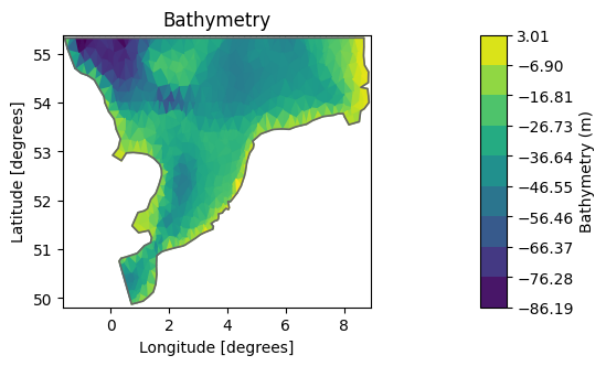
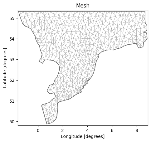
msh = mikeio.open("data/southern_north_sea.mesh")
msh
<Mesh>
number of nodes: 570
number of elements: 958
projection: LONG/LAT
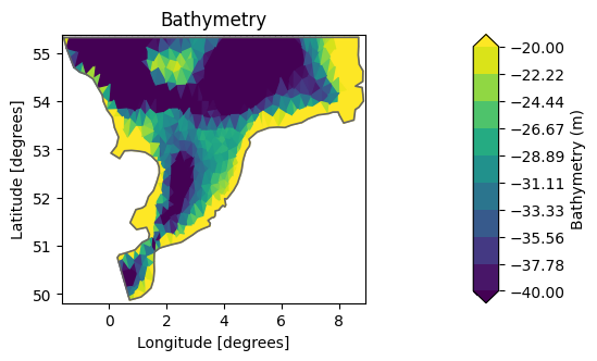
The default is to plot the elements and color them according to the bathymetry.
msh.plot();
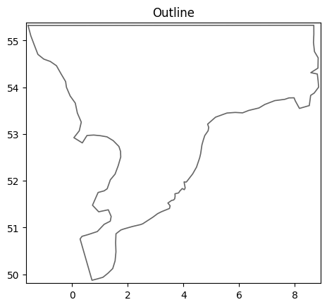
msh.plot.outline();
msh.plot.mesh();
Maybe we would like to higlight the bathymetric variations in some range, in this case in the -40, -20m range.
msh.plot(vmin=-40, vmax=-20);
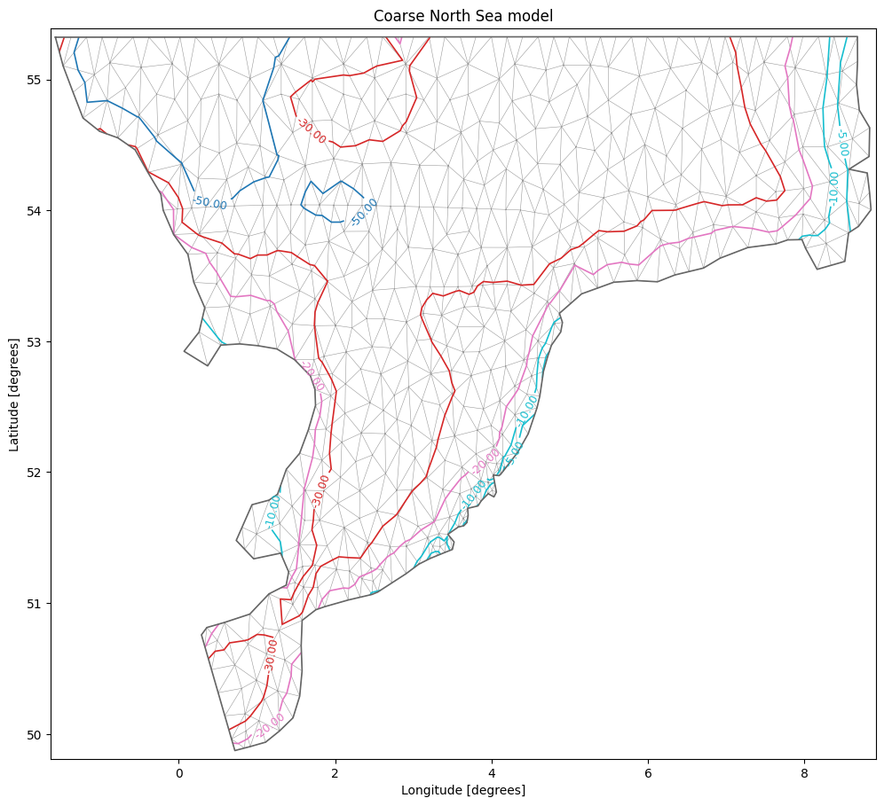
There are other options as well, such as explicit specification of which contour lines to show or choosing a specific colormap (matplotlib colormaps)
msh.plot.contour(show_mesh=True,
         levels=[-50,-30,-20,-10,-5], cmap="tab10",
         figsize=(12,12), title="Coarse North Sea model");
See more in the MIKE IO User guide section on Mesh for more Mesh operations (including shapely operations).