import modelskill as ms
Model skill visualisation#
fn = 'data/SW/HKZN_local_2017_DutchCoast.dfsu'
mr = ms.model_result(fn, name='HKZN_local', item=0)

obs = [ms.PointObservation('data/SW/HKZA_Hm0.dfs0', item=0, x=3.9, y=52.7, name="HKZA"),
        ms.PointObservation('data/SW/HKZA_Hm0.dfs0', item=0, x=3.8, y=52.5, name="HKZA_2"),
        ms.PointObservation('data/SW/HKZA_Hm0.dfs0', item=0, x=3.5, y=52.6, name="HKZA_3"),
        ms.PointObservation('data/SW/HKNA_Hm0.dfs0', item=0, x=4.2420, y=52.6887, name="HKNA"),
        ms.PointObservation('data/SW/HKNA_Hm0.dfs0', item=0, x=4.2, y=52.6, name="HKNA_2"),
        ms.PointObservation('data/SW/HKNA_Hm0.dfs0', item=0, x=4.3, y=52.7, name="HKNA_3"),
        ms.PointObservation("data/SW/eur_Hm0.dfs0", item=0, x=3.2760, y=51.9990, name="EPL"),
        ms.PointObservation("data/SW/eur_Hm0.dfs0", item=0, x=3.2, y=51.9, name="EPL_2"),
        ms.PointObservation("data/SW/eur_Hm0.dfs0", item=0, x=3.3, y=51.95, name="EPL_3")
]

cc = ms.match(obs=obs, mod=mr)
cc
/opt/hostedtoolcache/Python/3.13.12/x64/lib/python3.13/site-packages/mikeio/dataset/_dataset.py:505: FutureWarning: 'inplace' parameter is deprecated and will be removed in future versions. Use ds = ds.rename(...) instead.
  warnings.warn(
/opt/hostedtoolcache/Python/3.13.12/x64/lib/python3.13/site-packages/mikeio/dataset/_dataset.py:505: FutureWarning: 'inplace' parameter is deprecated and will be removed in future versions. Use ds = ds.rename(...) instead.
  warnings.warn(
/opt/hostedtoolcache/Python/3.13.12/x64/lib/python3.13/site-packages/mikeio/dataset/_dataset.py:505: FutureWarning: 'inplace' parameter is deprecated and will be removed in future versions. Use ds = ds.rename(...) instead.
  warnings.warn(
/opt/hostedtoolcache/Python/3.13.12/x64/lib/python3.13/site-packages/mikeio/dataset/_dataset.py:505: FutureWarning: 'inplace' parameter is deprecated and will be removed in future versions. Use ds = ds.rename(...) instead.
  warnings.warn(
/opt/hostedtoolcache/Python/3.13.12/x64/lib/python3.13/site-packages/mikeio/dataset/_dataset.py:505: FutureWarning: 'inplace' parameter is deprecated and will be removed in future versions. Use ds = ds.rename(...) instead.
  warnings.warn(
/opt/hostedtoolcache/Python/3.13.12/x64/lib/python3.13/site-packages/mikeio/dataset/_dataset.py:505: FutureWarning: 'inplace' parameter is deprecated and will be removed in future versions. Use ds = ds.rename(...) instead.
  warnings.warn(
/opt/hostedtoolcache/Python/3.13.12/x64/lib/python3.13/site-packages/mikeio/dataset/_dataset.py:505: FutureWarning: 'inplace' parameter is deprecated and will be removed in future versions. Use ds = ds.rename(...) instead.
  warnings.warn(
/opt/hostedtoolcache/Python/3.13.12/x64/lib/python3.13/site-packages/mikeio/dataset/_dataset.py:505: FutureWarning: 'inplace' parameter is deprecated and will be removed in future versions. Use ds = ds.rename(...) instead.
  warnings.warn(
/opt/hostedtoolcache/Python/3.13.12/x64/lib/python3.13/site-packages/mikeio/dataset/_dataset.py:505: FutureWarning: 'inplace' parameter is deprecated and will be removed in future versions. Use ds = ds.rename(...) instead.
  warnings.warn(
<ComparerCollection>
Comparers:
0: HKZA - Significant wave height [m]
1: HKZA_2 - Significant wave height [m]
2: HKZA_3 - Significant wave height [m]
3: HKNA - Significant wave height [m]
4: HKNA_2 - Significant wave height [m]
5: HKNA_3 - Significant wave height [m]
6: EPL - Significant wave height [m]
7: EPL_2 - Significant wave height [m]
8: EPL_3 - Significant wave height [m]
Data analysis#
cc.skill()
/opt/hostedtoolcache/Python/3.13.12/x64/lib/python3.13/site-packages/modelskill/metrics.py:344: RuntimeWarning: divide by zero encountered in scalar divide
  return 1 - SSr / SSt
| n | bias | rmse | urmse | mae | cc | si | r2 | |
|---|---|---|---|---|---|---|---|---|
| observation | ||||||||
| HKZA | 1 | 0.546863 | 0.546863 | 0.0 | 0.546863 | NaN | 0.0 | -inf |
| HKZA_2 | 1 | 0.527374 | 0.527374 | 0.0 | 0.527374 | NaN | 0.0 | -inf |
| HKZA_3 | 1 | 0.523389 | 0.523389 | 0.0 | 0.523389 | NaN | 0.0 | -inf |
| HKNA | 1 | 0.186511 | 0.186511 | 0.0 | 0.186511 | NaN | 0.0 | -inf |
| HKNA_2 | 1 | 0.164091 | 0.164091 | 0.0 | 0.164091 | NaN | 0.0 | -inf |
| HKNA_3 | 1 | 0.172111 | 0.172111 | 0.0 | 0.172111 | NaN | 0.0 | -inf |
| EPL | 1 | 0.518057 | 0.518057 | 0.0 | 0.518057 | NaN | 0.0 | -inf |
| EPL_2 | 1 | 0.474516 | 0.474516 | 0.0 | 0.474516 | NaN | 0.0 | -inf |
| EPL_3 | 1 | 0.508518 | 0.508518 | 0.0 | 0.508518 | NaN | 0.0 | -inf |
s = cc.skill()
type(s)
/opt/hostedtoolcache/Python/3.13.12/x64/lib/python3.13/site-packages/modelskill/metrics.py:344: RuntimeWarning: divide by zero encountered in scalar divide
  return 1 - SSr / SSt
modelskill.skill.SkillTable
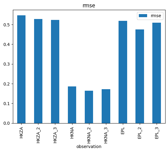
s.rmse.plot.bar();
s['urmse'].plot.line();
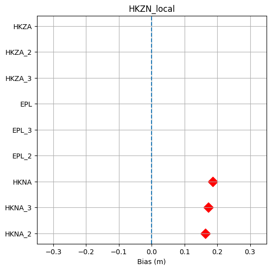
Custom plot#
All skill statistics are available in a dataframe, and in case you need a tailor-made plot, you can get data and use matplotlib to get exactly what you need.
import matplotlib.pyplot as plt
df = s.to_dataframe().sort_values('bias')
x = df.bias
y = df.index
plt.subplots(figsize=(6,6))
plt.scatter(x,y,marker='D',c='red',s=100)
plt.xlim(-0.35,0.35)
plt.axvline(0,linestyle='--')
plt.xlabel("Bias (m)")
plt.title(mr.name)
plt.grid()