Operational pilot¶

For the operational pilot, we have set up an operational-like development environment. The purpose of this environment is to have an experimental playground, where execution of the RTC robot can be scheduled as in the real-world operation system in a non-intrusive way.

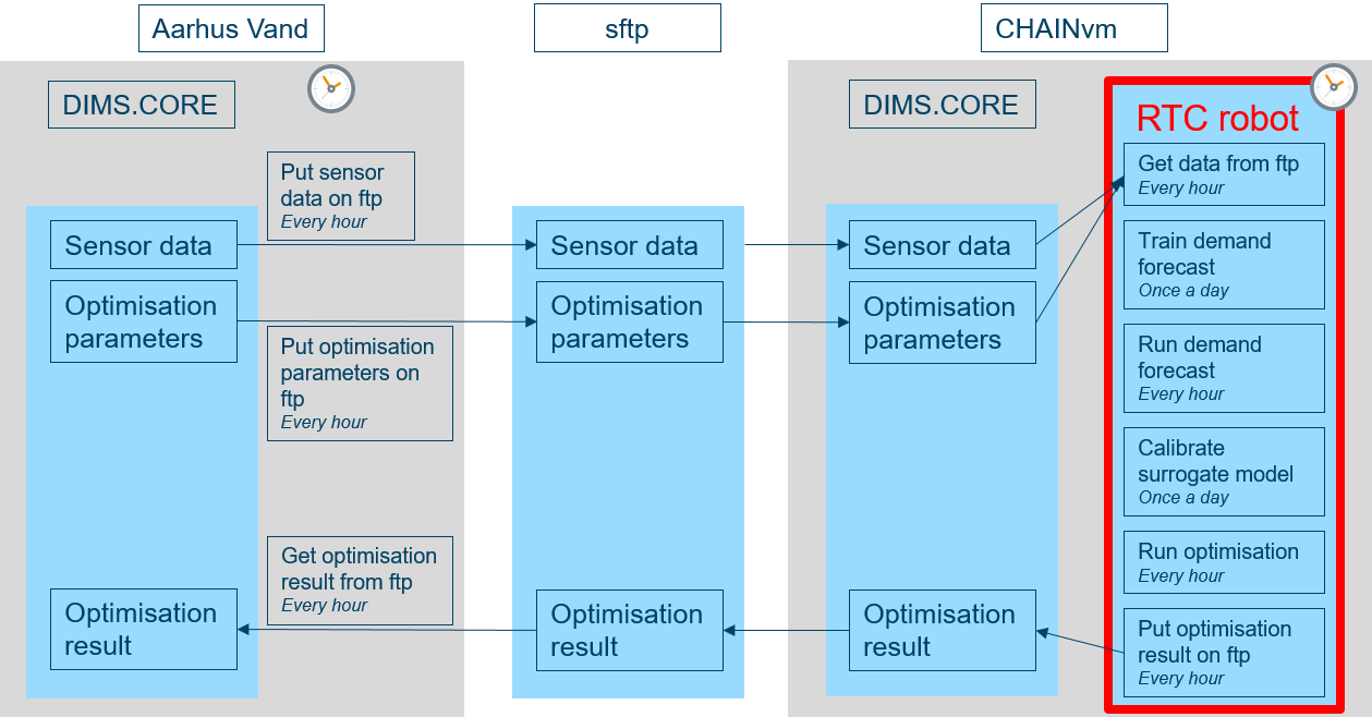
The operational-like development environment is set up on a virtual machine, henceforth referred to as CHAINvm. CHAINvm communicates with Aarhus Vand's operational system through an sftp-site. The communication flow is that Aarhus Vand puts sensor data on sftp, CHAINvm fetches the sensor data and use these as input to the RTC robot, which executes a model work-flow that results in optimised set-points for the waterworks. Finally the set-points are put on sftp for Aarhus Vand to pick up.

This workflow has been running hourly for the z80 pressure zone since April 2021. As a newly added feature, Aarhus Vand has the opportunity to manipulate selected parameters of the RTC robot by putting an additional file with parameters related to the optimisation on sftp along with the sensor data.

What's installed on CHAINvm¶

Software parts list¶

DIMS.CORE¶

DIMS.CORE is commercial DHI software, which serves as a repository for collected data and has a scheduler, which is used for timing data collection and model execution. DIMS.CORE needs an underlying database, on CHAINvm the free Microsoft SQL Server 2019 Express is installed.

Demand forecast model¶

The demand forecast model is a python package, which has been developed by the Alexandra Intitute as a part of the CHAIN project. The package contains three different machine learning models (seasonal, sarimax and gradient boosting) that are different models for the same task: based on the historical demand data, predict the demand for the forthcoming days.

It has a command line interface, through which it can be specified which task to execute (training or prediction) and which model to run. The models are configured in a text file, and read historical demand data from a .csv file

Controller¶

The controller is a python package, which has been developed by DHI as a part of the CHAIN project. The package contains tools for identifying and calibrating a simplified network model of the water distribution network, based on measurements of flow and pressure. The optimisation model itself is (so far) not included in the package but is a customised script on top of the package functionality.

The static data (the network layout) can be specified in a .csv file or encoded by a script. The dynamic data (boundary conditions) are connected to the network configuration, but have separate configuration files to keep track of units and aggregation of more boundary flows into one.

Optimisation solver¶

The controller uses the MOSEK solver. MOSEK is an industry standard commercial solver (which is not affiliated with any of the project partners).

Software installation¶

The demand forecast model and the controller are installed from their respective source, each of them in their own virtual environment. This ensures that their dependencies do not interfere, and that the models are executed completely isolated from each other. The source codes reside inside Alexandra Institute and DHI internal code repositories.

What happens during a computational cycle¶

There are two heartbeats of the computational cycle

Every hour the RTC robot calculates the set-points for the waterworks for the next 48 h
Once a day, the models of the RTC robot are retrained/recalibrated

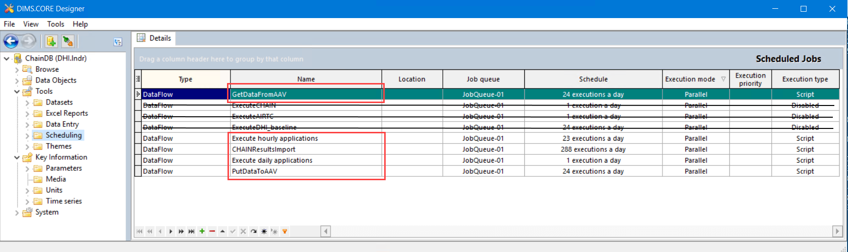
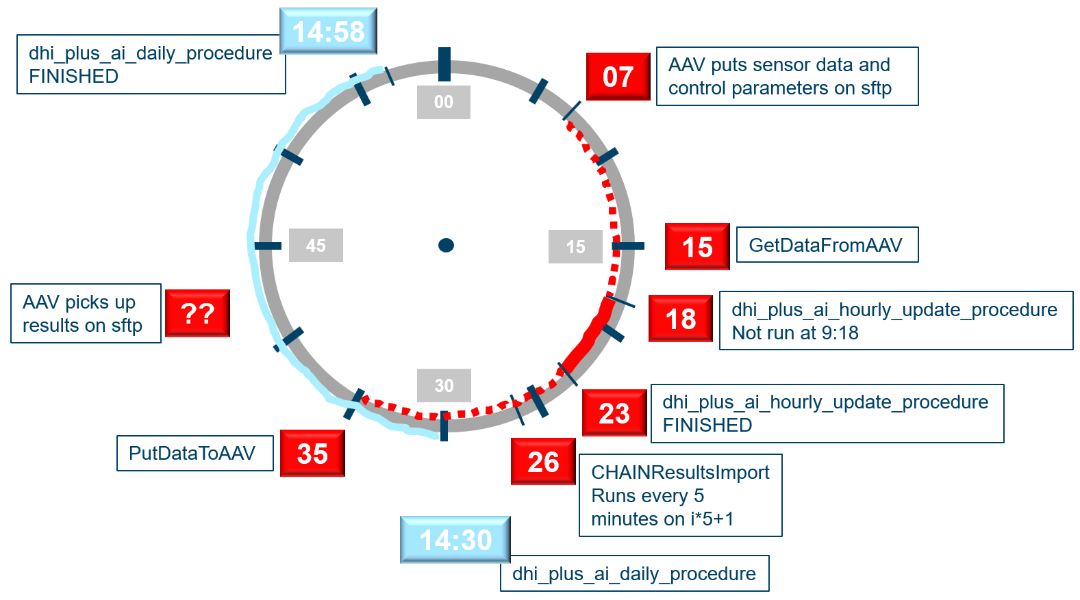
The timing of the execution is controlled by DIMS.CORE's scheduler. A screen dump from the scheduler is shown below. The active scripts are shown in red boxes, and the minute of the hour they are executed is shown in red on the "clock". The once-a-day execution starts at 9:30, and its time extent is visualised by the blue line.

Hourly tasks¶

The scheduling of the hourly tasks has been set up to accommodate experimental runs that were not timed in advance, therefore some idle time occurs. For the hourly schedule, mostly idle time is marked by a dashed red line, whereas the solid red line shows the period with no slack. The transfer of data from Aarhus Vand at minute 07 happens within seconds, and so does the retrieval on CHAINvm at minute 15. The actually time-consuming part of the RTC robot happens during 5 minutes from minute 18 to 23. This is the part that prepares the data for the models and then runs the demand prognosis and the optimisation.

Most notably, it is NOT the execution of the models that takes most of the time, in total the models finish in tens of seconds. The models in question are gradient boosting demand prognosis and two versions of the optimisation (see Parallel playground setups). The most of the time is consumed by extracting and writing 100 days of data in one-minute resolution - a data set, which is an input to the demand prognosis. The file is about 45MB and the operation of extracting from DIMS.CORE and writing to a .csv-file takes about 3.5 minutes. We are confident that this bottleneck can be dealt with, and that we can squeeze the workflow so that the PutDataToAAV task (currently at minute 35) can take place before minute 15.

Daily task¶

Re-train demand prognosis models¶

Once a day, all of the three demand prognosis models are re-trained, based on the latest 100 days' data. Execution of the entire job takes 28 minutes, from 14:30 to 14:58, and it has been scheduled to start at minute 30 in order not to interfere with execution of the hourly tasks.

Take a look at the log from the training (open in a new tab to see details).

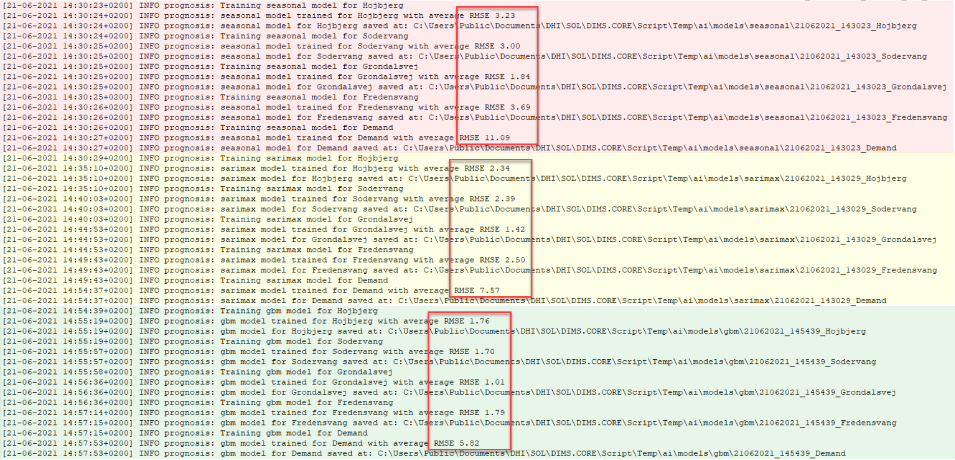
The time consuming part is the training of the sarimax model (~25 min) and the gradient boosting model (~5 min), whereas the seasonal model in comparison is quick (few seconds). The training scales linearly with the number of demand sections, ~5 min per section for sarimax, ~1 min per section for gradient boosting. The colour-coding relates to the magnitude of the training RMSE for each model. Gradient boosting has the lowest RMSE (green), next comes sarimax (yellow) and somewhat higher comes the seasonal model (red). This is an argument to prefer the gradient boosting model: lowest RMSE, with a training time which is much less than for sarimax. The seasonal model only competes on training time.

Note that all three types of demand models are trained every day, but the current versions of the RTC robot are configured to use the gradient boosting model. This is also a benefit of the experimental environment on CHAINvm.

Re-calibrate network model¶

Re-calibration of the network's resistance parameters is also a part of the daily task. Note that even if the calibration is not carried out, the network model's linearisation is still updated each time the hourly task runs, because the coefficients of the linearised pressure loss model, $\alpha |q_0|$ , are calculated using the flow at the current operating point as $q_0$ .

Parallel playground setups¶

One of the advantages of having a development environment as CHAINvm is the possibility to run more configurations of the models in parallel. At the end of the project two different optimisation models are running. The two optimisation models use the same network layout, "micro", which takes pressure at critical locations into account. One optimisation model is dedicated to Aarhus Vand's experiments with choice of the optimisation parameters, the other to DHI's experiments.