Data handling

The boundary conditions for the mpc are vectors with a length defined by the control horizon. Measurements from the system must be modified to a unit and sampling rate that matches the model definitions. Other key features in the data handling process includes:

• Filter noise from the measurements.
• Add elevation to pressure measurements.
• Identify the minimal modification for the demand and water productions to solve a mass balance across the disrict.
• Solve an inner massbalance to create data for each flow state.

Pipe water pressure, when measured, is overpressure or surplus pressure at the sensor location, which changes relative to the elevation. The model operates with a different notion of pressure; one that is absolute with respect to a reference shared by all pressure states.

Resampling and noise filtering

• Resampling. Filters high frequency noise and aligns the sampling to the desired discretization of the model. The default in this operation is that several samples inside a resampled interval is averaged. Assuming that the measurement disturbances are white noise, this is also an effective filtration operation.

• Polynomial filtering. Savitsky-Golay filtration corrects each data point, using the values of the neighbours symmetrically forward and backwards in the time axis. This too eliminates a significant amount of noise at the specified sampling.

Measurement processing

• Correct for elevation (pressure). Each pressure sensor measures excess pressure above the sensor's elevation. The pressure measurements are aligned to a shared reference by adding each sensor's elevation to the recorded excess pressure.
• Unit conversion. Convert measured pressure to meter water. It is preferred that input to the model use the basic units. For models with elevated storage, this is required, as these are often measured by the level of water surface.
• Add bias to pressure measurements. Bias can be included to adjust the pressure measurements to comply with the flow direction. In some cases, a pressure measurement can't be acquired at exactly the desired location (often junction). Then the bias is used to account for the elevation difference between the measured point and model point.

Mass balance correction

Outer massbalance

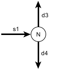
Part of satisfying the continuity requirement for the distribution system flows, is that the boundary conditions sum to zeros. This is equivalent to contracting the system graph to a single node, so only lateral flows remain.

This problem has some differences to what was described in Section 3:

• It is required that each lateral flow has an observation.
• There is no minimum flow requirement.

The system is solved as an e quality constrained quadratic program:

$$\begin{matrix} \min\limits_{x} f(x)= \frac{1}{2} || x - q_{lat} ||_2^2 \\ s.t. \\ \sum x = 0 \end{matrix}$$

The general form is:

$$\begin{matrix} \min\limits_{x} f(x)= \frac{1}{2} || A_{ss} x - b_{ss} ||_2^2 \\ s.t. \\ A_c x=b_c \end{matrix}$$

where ss denotes state space and c denotes constraint.

In the program formulation, compared to the regular form: , the A matrix is omitted. With a single node system, there is no system dynamics, so the internal states matrix, A, is the identity matrix. With the single equality constraint, the KKT conditions are defined:

$$\begin{bmatrix} G & -A \\ -A^T & 0 \end{bmatrix} \begin{bmatrix} x \\ y \end{bmatrix} = \begin{bmatrix} g \\ b \end{bmatrix}$$

where A is the constraint matrix, $\begin{bmatrix} 1 & 1 & 1 \end{bmatrix}$ and b is the right-hand side constraint, 0. G and g, are derived from the QP on the internal states:

$$\begin{matrix} G = A^T_{ss}A_{ss} = I^TI = I \\ g = -A^T_{ss}b_{ss} = - \begin{bmatrix} -s_1 \\ d_3 \\ d_4 \end{bmatrix} = \begin{bmatrix} s_1 \\ -d_3 \\ -d_4 \end{bmatrix} \end{matrix}$$

where the signs are given depending if the lateral flow is a source or sink, see Figure XX. The solver scheme should largely be chosen based on the properties of the G matrix, since it must be inverted. In the specific use here, the G matrix is the identity, so inverting is trivial.

Inner massbalance

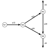
• The inner mass balance computes the flow through all pipes in the desired model by setting up a mass balance for each node.
• Pressure loss for each pipe can optionally be included as bounds to the output flow: A positive pressure loss will have only positive flow in the feasible region and vice versa.
• In the case that some of the pipes have measured flow, this information can be included, weighing the solution towards the observation. Note, that the given pipe flow is not hard constrained to the observation, as the observation might be subject to measurement uncertainty.
• When loops are present, but with insufficient (or none) flow sensors, the flow direction will be driven towards the ‘least energy’ state. That is the solution where the flows are closest to zero, in either positive or negative direction.
• The calculation of flows in edges is made before the resistance on the edges is calculated. The implicit assumption of the inner mass balance is that all edges have equal resistance, which is the best approximation at this stage in the workflow.

$$\begin{bmatrix} -1 & & & \\ 1 & -1 & -1 & \\ & 1 & & -1 \\ & & 1 & 1 \\ 1 & & & \\ & & 1 & \end{bmatrix} \begin{bmatrix} q_{12} \\ q_{23} \\ q_{24} \\ q_{34} \\ \\ \end{bmatrix} = \begin{bmatrix} -s_1 \\ 0 \\ d_3 \\ d_4 \\ m_{12} \\ m_{24} \end{bmatrix}$$

The first four rows are the mass balance in the nodes, the two last rows specify the two links with measured flows. This system is overdetermined, for instance the link q_12 should both fulfill the node balance (first row) and equal the measurement (fifth row). The task is to determine the flows that both keeps the node’s mass balances as close to zero as possible flows and is close to the measurement (where such exist). The system can be “solved” as an ordinary least squares problem where the deviation between left-hand side and right-hand side is minimized:

$$\min || Ax - b ||^2_2$$