from mikeio1d import Res1D
res = Res1D('../data/network.res1d')
res_catchments = Res1D('../data/catchments.res1d')
res_river = Res1D('../data/network_river.res1d')Locations
Locations are where model results exist in the Network. The main location types are nodes, reaches, and catchments. Structures are locations too.
Data structures
There are two main data structures for locations: location collections (ResultLocations) and single locations (ResultLocation).
Location collections
Access location collections from a Res1D object. Each collection shows available quantities and location IDs. Structures have a collection too, covered below.
res.nodes
<ResultNodes> (119)
Quantities (1)
- Water level (m)
Derived Quantities (3)
- NodeFlooding
- NodeWaterDepth
- NodeWaterLevelAboveCritical
res.reaches
<ResultReaches> (118)
Quantities (2)
- Water level (m)
- Discharge (m^3/s)
Derived Quantities (6)
- ReachAbsoluteDischarge
- ReachFilling
- ReachFlooding
- ReachQQManning
- ReachWaterDepth
- ReachWaterLevelAboveCritical
res_catchments.catchments
<ResultCatchments> (31)
Quantities (5)
- Total Runoff (m^3/s)
- Actual Rainfall (m/s)
- Zink, Load, RR (kg/s)
- Zink, Mass, Accumulated, RR (kg)
- Zink, RR (mg/l)
Derived Quantities (0)
Note
Gridpoints only exist as single locations on a reach, and have no collection.
Single locations
Access a single location by indexing its respective collection with its unique ID. Each location shows available quantities and static properties.
res.nodes['1']
<Manhole: 1>
Attributes (8)
- id: 1
- type: Manhole
- xcoord: -687934.6000976562
- ycoord: -1056500.69921875
- ground_level: 197.07000732421875
- bottom_level: 195.0500030517578
- critical_level: inf
- diameter: 1.0
Quantities (1)
- Water level (m)
Derived Quantities (3)
- NodeFlooding
- NodeWaterDepth
- NodeWaterLevelAboveCritical
res.reaches['100l1']
<Reach: 100l1>
Attributes (9)
- name: 100l1
- length: 47.6827148432828
- start_chainage: 0.0
- end_chainage: 47.6827148432828
- n_gridpoints: 3
- start_node: 100
- end_node: 99
- height: 0.30000001192092896
- full_flow_discharge: 0.12058743359507902
Quantities (2)
- Water level (m)
- Discharge (m^3/s)
Derived Quantities (6)
- ReachAbsoluteDischarge
- ReachFilling
- ReachFlooding
- ReachQQManning
- ReachWaterDepth
- ReachWaterLevelAboveCritical
# gridpoint on reach 100l1 at chainage 23.841
res.reaches['100l1']['23.841']
<ResultGridPoint>
Attributes (5)
- reach_name: 100l1
- chainage: 23.8413574216414
- xcoord: -687897.8000488281
- ycoord: -1056390.4503479004
- bottom_level: 195.0500030517578
Quantities (1)
- Discharge (m^3/s)
Derived Quantities (0)
Tip
Gridpoints can also be indexed by number instead of chainage. For example:
res.reaches['100l1'][0]  # first gridpoint
res.reaches['100l1'][-1] # last gridpointres_catchments.catchments['100_16_16']
<Catchment: 100_16_16>
Attributes (3)
- id: 100_16_16
- area: 22800.0
- type: Kinematic Wave
Quantities (5)
- Total Runoff (m^3/s)
- Actual Rainfall (m/s)
- Zink, Load, RR (kg/s)
- Zink, Mass, Accumulated, RR (kg)
- Zink, RR (mg/l)
Derived Quantities (0)
Quantities
Quantities are the actual model results. Each single location or location collection has associated quantities.
res.nodes.WaterLevel<QuantityCollection (119): Water level (m)>res.nodes['1'].WaterLevel<Quantity: Water level (m)>
TipCan’t find a which location a quantity belongs to?
The Network structure is generic and applies across different domains (e.g. collection systems, water distribution, rivers). Sometimes this can be challenging to find a particular result. Here are some examples of result types mapped onto this structure.
| Location | Example quantities |
|---|---|
| Nodes | Water level (e.g. manhole, basin, outlet, junction) |
| Reaches | Discharge (e.g. pipes, pumps, weirs) |
| Water level (e.g. at specific chainages) | |
| Structures | Discharge (e.g. weirs, gates, bridges, pumps) |
| Flow area and velocity in structure | |
| Catchments | Catchment discharge |
| Total runoff | |
| Global | Water balance |
| User defined variable types |
Refer to the Quantities page for more information on how to read and plot the returned quantities.
Static attributes
Each location has a set of static attributes.
res.nodes['1'].ground_level197.07000732421875Reading data
All result data for a single location or location collection can be read into a pandas DataFrame.
df = res.reaches['100l1'].read()
df.head()| WaterLevel:100l1:0 | WaterLevel:100l1:47.6827 | Discharge:100l1:23.8414 | |
|---|---|---|---|
| 1994-08-07 16:35:00.000 | 195.441498 | 194.661499 | 0.000006 |
| 1994-08-07 16:36:01.870 | 195.441498 | 194.661621 | 0.000006 |
| 1994-08-07 16:37:07.560 | 195.441498 | 194.661728 | 0.000006 |
| 1994-08-07 16:38:55.828 | 195.441498 | 194.661804 | 0.000006 |
| 1994-08-07 16:39:55.828 | 195.441498 | 194.661972 | 0.000006 |
df = res.reaches.read()
df.head()| WaterLevel:100l1:0 | WaterLevel:100l1:47.6827 | WaterLevel:101l1:0 | WaterLevel:101l1:66.4361 | WaterLevel:102l1:0 | WaterLevel:102l1:10.9366 | WaterLevel:103l1:0 | WaterLevel:103l1:26.0653 | WaterLevel:104l1:0 | WaterLevel:104l1:34.4131 | ... | Discharge:93l1:24.5832 | Discharge:94l1:21.2852 | Discharge:95l1:21.9487 | Discharge:96l1:14.9257 | Discharge:97l1:5.71207 | Discharge:98l1:8.00489 | Discharge:99l1:22.2508 | Discharge:9l1:5 | Discharge:Weir:119w1:0.5 | Discharge:Pump:115p1:41.214 | |
|---|---|---|---|---|---|---|---|---|---|---|---|---|---|---|---|---|---|---|---|---|---|
| 1994-08-07 16:35:00.000 | 195.441498 | 194.661499 | 195.931503 | 195.441498 | 193.550003 | 193.550003 | 195.801498 | 195.701508 | 197.072006 | 196.962006 | ... | 0.000004 | 0.000003 | 0.000001 | 0.000005 | 0.000013 | 0.000003 | 0.000002 | 0.000031 | 0.0 | 0.0 |
| 1994-08-07 16:36:01.870 | 195.441498 | 194.661621 | 195.931503 | 195.441605 | 193.550140 | 193.550064 | 195.801498 | 195.703171 | 197.072006 | 196.962051 | ... | 0.000004 | 0.000003 | 0.000001 | 0.000005 | 0.000010 | 0.000003 | 0.000002 | 0.000031 | 0.0 | 0.0 |
| 1994-08-07 16:37:07.560 | 195.441498 | 194.661728 | 195.931503 | 195.441620 | 193.550232 | 193.550156 | 195.801498 | 195.703400 | 197.072006 | 196.962082 | ... | 0.000004 | 0.000003 | 0.000001 | 0.000005 | 0.000010 | 0.000003 | 0.000002 | 0.000033 | 0.0 | 0.0 |
| 1994-08-07 16:38:55.828 | 195.441498 | 194.661804 | 195.931503 | 195.441605 | 193.550369 | 193.550308 | 195.801498 | 195.703690 | 197.072006 | 196.962112 | ... | 0.000004 | 0.000003 | 0.000001 | 0.000005 | 0.000009 | 0.000003 | 0.000002 | 0.000037 | 0.0 | 0.0 |
| 1994-08-07 16:39:55.828 | 195.441498 | 194.661972 | 195.931503 | 195.441605 | 193.550430 | 193.550369 | 195.801498 | 195.703827 | 197.072006 | 196.962128 | ... | 0.000004 | 0.000003 | 0.000001 | 0.000005 | 0.000009 | 0.000003 | 0.000002 | 0.000039 | 0.0 | 0.0 |
5 rows × 376 columns
A single location can also be narrowed down to some of its quantities. The same quantities argument is taken by add, plot, to_csv, to_dfs0 and to_txt.
df = res.reaches['100l1'].read(quantities='Discharge')
df.head()| Discharge:100l1:23.8414 | |
|---|---|
| 1994-08-07 16:35:00.000 | 0.000006 |
| 1994-08-07 16:36:01.870 | 0.000006 |
| 1994-08-07 16:37:07.560 | 0.000006 |
| 1994-08-07 16:38:55.828 | 0.000006 |
| 1994-08-07 16:39:55.828 | 0.000006 |
res.reaches['100l1'].plot(quantities='WaterLevel')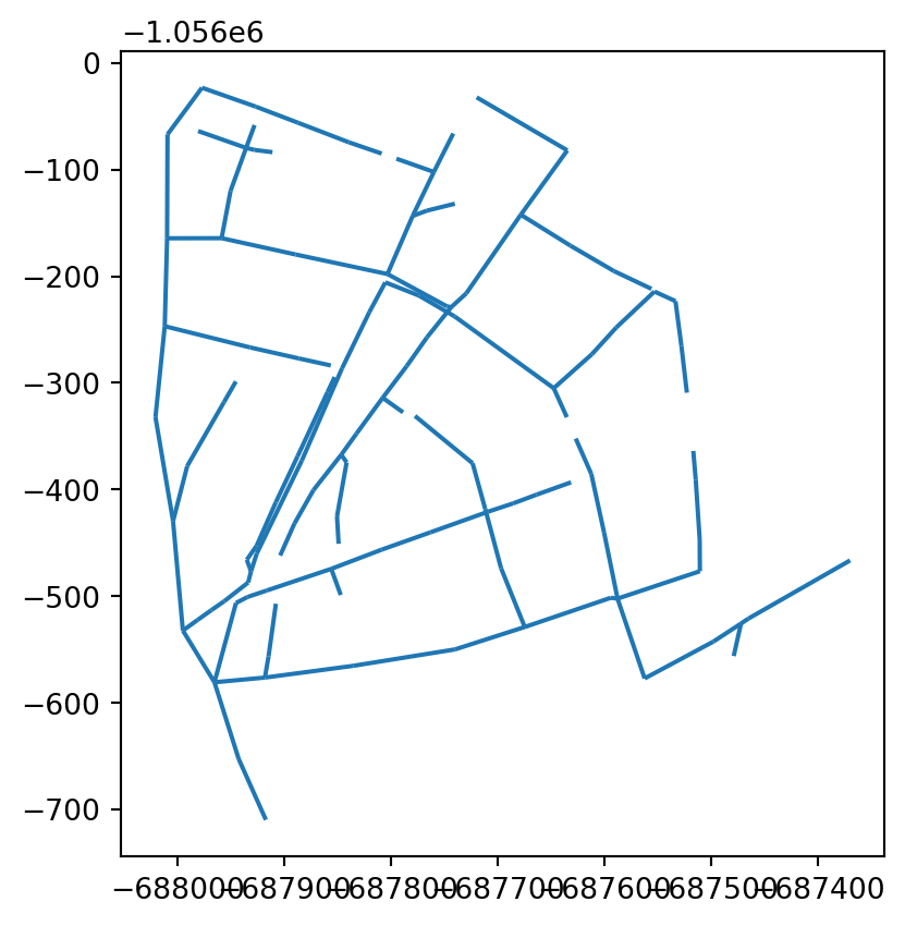
Structures
Structure results are accessed through the structure collection, keyed by structure ID. Each structure is its own location, so structures at the same reach chainage stay apart.
res_river.structures
<ResultStructures> (10)
Quantities (6)
- Flow velocity in structure: W_left_1_1 (Broad Crested Weir) (m/s)
- Flow area in structure: W_left_1_1 (Broad Crested Weir) (m^2)
- Discharge in structure: W_left_1_1 (Broad Crested Weir) (m^3/s)
- Control strategy ID: W_left_1_1 (Broad Crested Weir) (Integer)
- Discharge (m^3/s)
- Gate level: Outer Gates (Underflow Gate) (m)
Derived Quantities (0)
Access a single structure by indexing the collection with its ID. The header and type attribute show its reach (river), and chainage its position on it. Here DamCrest, Outer Gates and Inner Gates share chainage 53727.17.
res_river.structures['Outer Gates']
<river: Outer Gates>
Attributes (3)
- id: Outer Gates
- type: river
- chainage: 53727.17
Quantities (5)
- Flow velocity in structure: Outer Gates (Underflow Gate) (m/s)
- Flow area in structure: Outer Gates (Underflow Gate) (m^2)
- Gate level: Outer Gates (Underflow Gate) (m)
- Discharge in structure: Outer Gates (Underflow Gate) (m^3/s)
- Control strategy ID: Outer Gates (Underflow Gate) (Integer)
Derived Quantities (0)
Reading a quantity from the collection gives one column per structure.
df = res_river.structures.DischargeInStructure.read()
df.describe().T| count | mean | std | min | 25% | 50% | 75% | max | |
|---|---|---|---|---|---|---|---|---|
| DischargeInStructure:W_left_1_1:link_basin_left:46 | 73.0 | 4.447620 | 5.618053 | -2.671227e+00 | 0.000000 | 0.944011 | 9.329815 | 13.542682 |
| DischargeInStructure:link_links_1_2_LinkChannel:link_basin_left1_2:29.3 | 73.0 | 0.000000 | 0.000000 | 0.000000e+00 | 0.000000 | 0.000000 | 0.000000 | 0.000000 |
| DischargeInStructure:link_links_2_2_LinkChannel:link_basin_left2_2:34.5 | 73.0 | 0.000000 | 0.000000 | 0.000000e+00 | 0.000000 | 0.000000 | 0.000000 | 0.000000 |
| DischargeInStructure:W_right:link_basin_right:18 | 73.0 | 5.583869 | 3.809939 | 0.000000e+00 | 0.036112 | 6.468229 | 8.696654 | 11.018318 |
| DischargeInStructure:bridge1:river:53126.8 | 73.0 | 61.389126 | 26.613249 | 0.000000e+00 | 69.116371 | 74.444443 | 75.857216 | 77.608521 |
| DischargeInStructure:DamCrest:river:53727.2 | 73.0 | 0.000000 | 0.000000 | 0.000000e+00 | 0.000000 | 0.000000 | 0.000000 | 0.000000 |
| DischargeInStructure:Outer Gates:river:53727.2 | 73.0 | 0.000000 | 0.000000 | 0.000000e+00 | 0.000000 | 0.000000 | 0.000000 | 0.000000 |
| DischargeInStructure:Inner Gates:river:53727.2 | 73.0 | 58.195927 | 28.547558 | -1.875944e-20 | 57.831062 | 59.101318 | 59.609913 | 100.247269 |
| DischargeInStructure:bridge2:river:54715 | 73.0 | 76.074913 | 28.324549 | 0.000000e+00 | 76.470184 | 85.356270 | 93.048927 | 100.058662 |
| DischargeInStructure:bridge3:river:54812.9 | 73.0 | 76.233047 | 28.184683 | 0.000000e+00 | 76.412148 | 85.804459 | 93.077385 | 100.017456 |
A structure can also be accessed as an attribute. Characters that aren’t valid in a Python name are replaced by underscores, so Inner Gates becomes Inner_Gates. Indexing with the ID always works, whatever characters it contains.
res_river.structures.Inner_Gates.FlowVelocityInStructure.plot()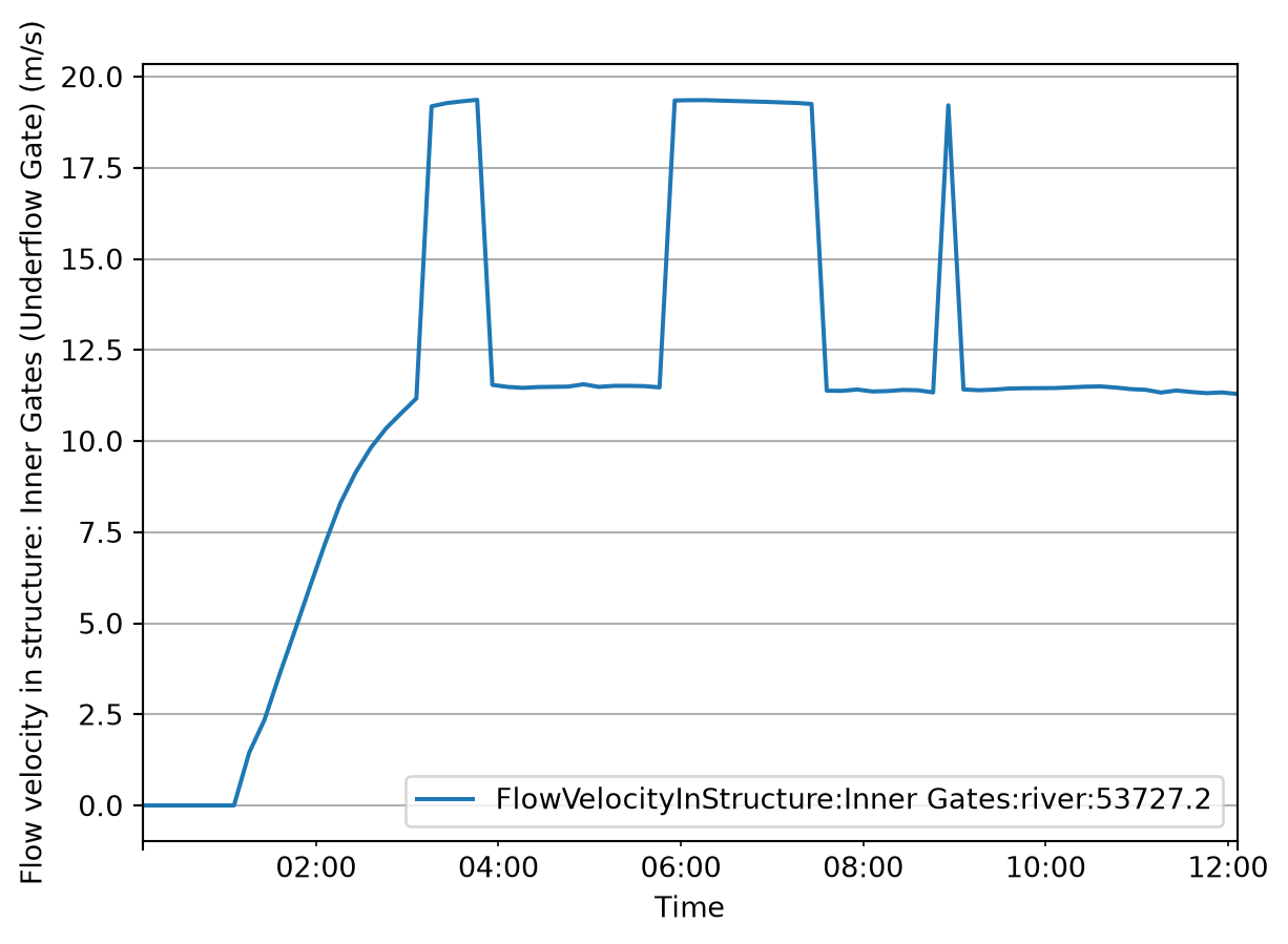
Structure IDs that start with a digit get an s_ prefix when accessed as an attribute. For example, weir 119w1 in network.res1d:
res.structures.s_119w1.Discharge.plot() # same as res.structures['119w1'].Discharge.plot()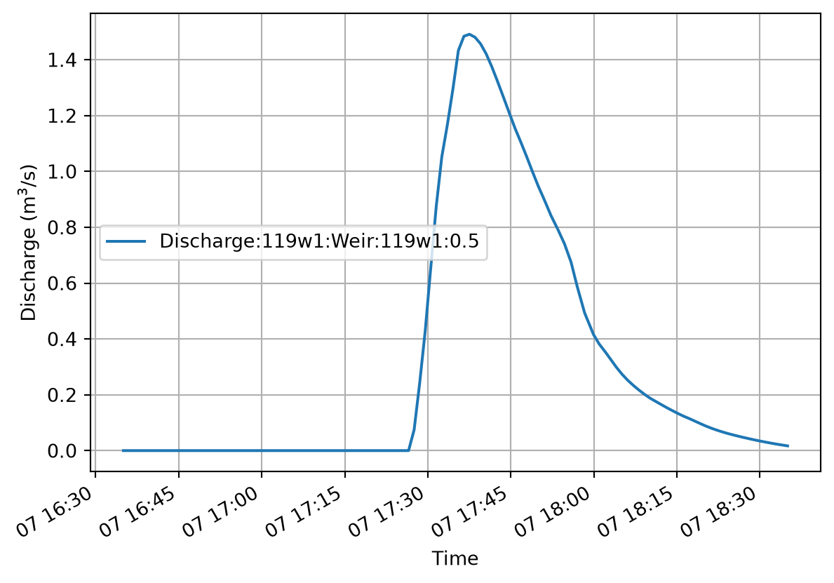
Structure results are also part of a full read, in the Structure group. With column_mode='compact' the columns are a MultiIndex of quantity, group, name, chainage and tag, which the m1d accessor can filter.
df = res_river.read(column_mode='compact')
df = df.m1d.query("group == 'Structure' and quantity == 'DischargeInStructure'")
df.tail()| quantity | DischargeInStructure | |||||||||
|---|---|---|---|---|---|---|---|---|---|---|
| group | Structure | |||||||||
| name | W_left_1_1 | link_links_1_2_LinkChannel | link_links_2_2_LinkChannel | W_right | bridge1 | DamCrest | Outer Gates | Inner Gates | bridge2 | bridge3 |
| chainage | 46.00 | 29.30 | 34.50 | 18.00 | 53126.75 | 53727.17 | 53727.17 | 53727.17 | 54715.00 | 54812.90 |
| tag | link_basin_left | link_basin_left1_2 | link_basin_left2_2 | link_basin_right | river | river | river | river | river | river |
| 2000-02-18 11:26:00 | 0.944011 | 0.0 | 0.0 | 5.192532 | 75.068871 | 0.0 | 0.0 | 58.953537 | 77.256615 | 77.207466 |
| 2000-02-18 11:36:00 | -0.811433 | 0.0 | 0.0 | 3.760968 | 73.730675 | 0.0 | 0.0 | 58.735832 | 76.470184 | 76.412148 |
| 2000-02-18 11:46:00 | -2.627501 | 0.0 | 0.0 | 3.810924 | 72.652916 | 0.0 | 0.0 | 58.578617 | 75.564018 | 75.549805 |
| 2000-02-18 11:56:00 | -2.143913 | 0.0 | 0.0 | 3.728211 | 72.600952 | 0.0 | 0.0 | 58.678886 | 74.693275 | 74.699257 |
| 2000-02-18 12:06:00 | -2.142947 | 0.0 | 0.0 | 3.013645 | 71.983345 | 0.0 | 0.0 | 58.462067 | 73.794426 | 73.775215 |
Note
In collection system files, each structure also has its own reach, named by type and ID. For example, pump 115p1 is both res.structures['115p1'] and res.reaches['Pump:115p1'].
GeoDataFrames
Locations collections can be extracted into a GeoDataFrame, both with and without quantities.
gdf = res.reaches.to_geopandas()
gdf.plot()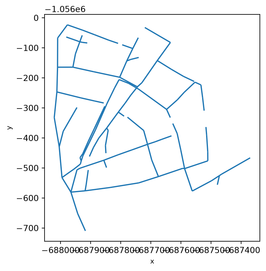
gdf = res.reaches.to_geopandas(agg='max')
gdf.plot(column='max_Discharge', linewidth=3, cmap='RdYlGn_r', legend=True)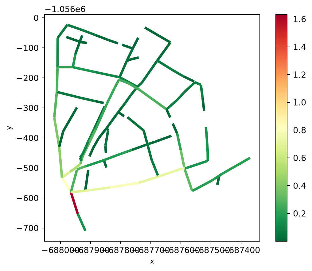
Examples
Tip
There are also several notebook examples available on our GitHub repositoryhttps://github.com/DHI/mikeio1d/tree/main/notebooks.