Network

A fundamental concept of MIKE IO 1D is the structure of a Network. Understanding its basic components is essential for working with the library.

Overview

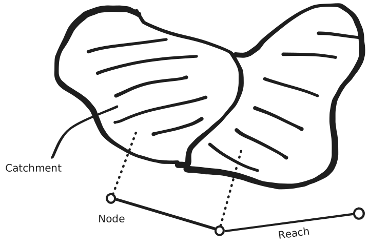
Networks consist of several elements: reaches, grid points, nodes, and catchments.

Reaches

Reaches have many synonyms within different domain applications. In collection systems they are often called links or pipes. In river models they are called branches, streams, canals or channels. In graph and network theory they are called links or edges. Reaches contains several ‘grid points’ along their path, and are bounded by nodes.

Grid Points

Grid points are the computational points along a reach. A flow model has different types of grid points:

H grid point: contains water level and an associated cross section.
Q grid point: contains discharge or flow velocity.
Structure grid point: calculates discharge over a structure depending on the water levels on each side of the structure.

Results for structures are read as their own location type (see Structures).

Nodes

Nodes are connected together by reaches. Nodes can represent different entities: manholes, basins, outlets, and junction nodes. They may or may not have a volume.

Catchments

Catchments are areas connected to either nodes or grid points, and act as boundary conditions for inputting loads to the network.

Reading a network as a graph

The mikeio1d.network module reads a result file into a graph of these elements. Each reach becomes a chain — its start node, its breakpoints in order, its end node — and every edge carries the distance between its two ends, where that is known. A location keeps the name the model gave it, a node id or a reach and a position along it, and the network is addressed by those names throughout. to_networkx() gives the graph, labelled with integers, each node carrying its name as the address attribute; resolve() gives the integer for a name, as NetworkLocation.graph_node. A graph node is not a model node: every location has one, a breakpoint too, and a model node is always named by its id. The graph is undirected, and each call builds a new one, which the caller is free to edit.

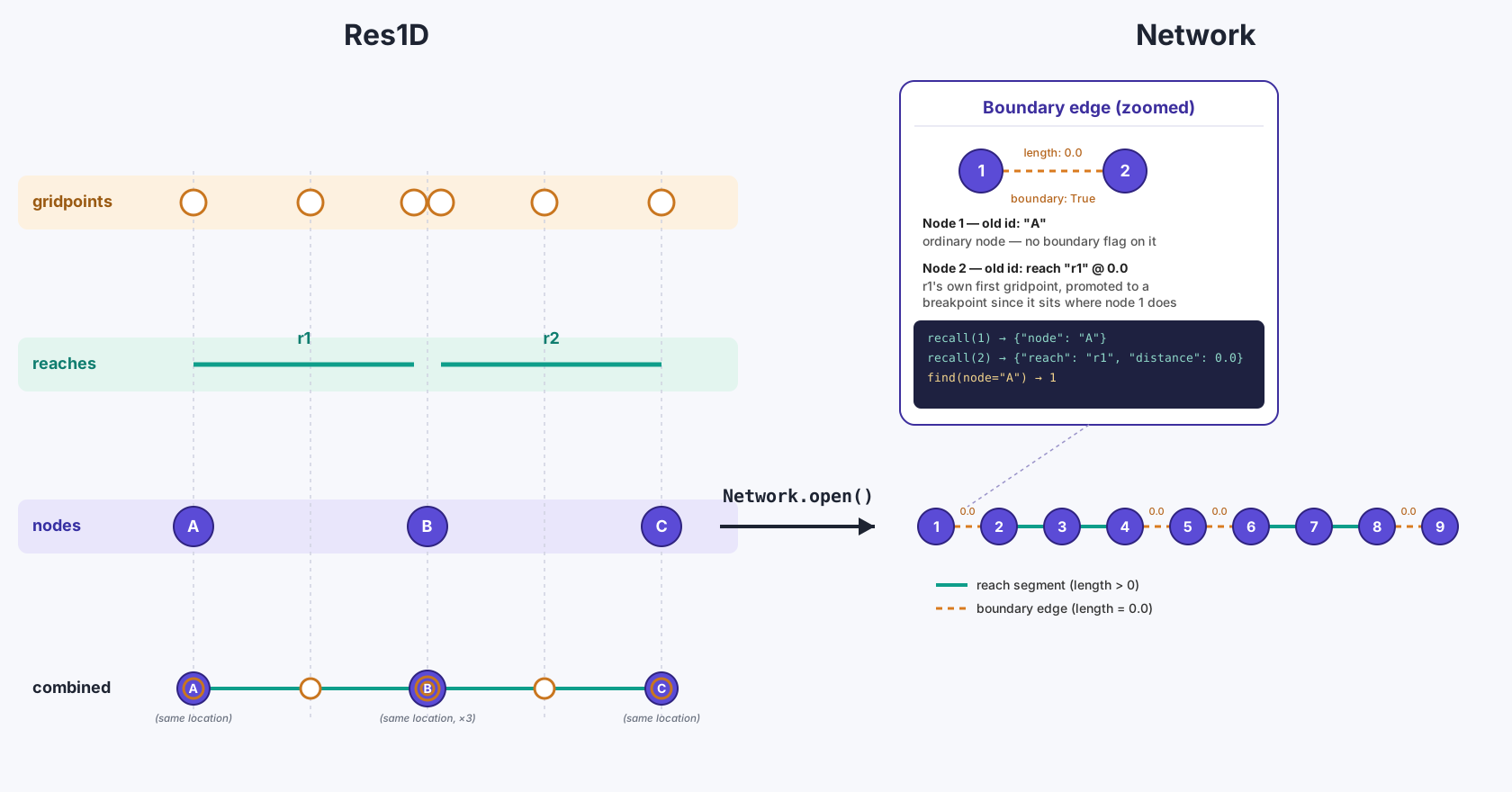
A reach’s own first and last grid point sit exactly where the reach’s nodes do, so each is joined to its node by an edge of length `0.0` flagged `boundary`. Drawn for a MIKE network: a link-node model such as EPANET has one synthetic grid point per reach, which is placed at both ends instead.

A boundary edge is free to cross

length=0.0 is a valid weight, so a length-weighted networkx call treats a boundary edge as a free hop rather than refusing it — unlike an edge whose length is unknown, which carries None. Filter on boundary where the distance should count only real reach segments.

The module needs the network extra:

pip install mikeio1d[network]

Reading only what you need

Network.open reads the header and the topology, and no timeseries:

from mikeio1d.network import Network

network = Network.open("model.res1d")

The network then answers from the file header and its own breakpoints, still without reading any:

network.period                                     # (start, end)
network.quantities                                 # {'WaterLevel': 'm', 'Discharge': 'm^3/s'}
network.resolve("manhole_12")                      # NetworkLocation(address=..., quantities=(...), graph_node=...)
network.addresses(reach="100l1", quantity="Discharge")

resolve() returns None for a location the network does not have, rather than raising, so a caller can ask before committing to a read. Give it a position_tol to snap a measured chainage onto the model’s:

network.resolve(("100l1", 23.8), position_tol=0.1)
# NetworkLocation(address=('100l1', 23.8413574216414), quantities=('Discharge',), graph_node=3)

A result’s grid is often staggered: on 100l1 the water level sits at 0.0 and 47.68 and the discharge at 23.84 between them. Give resolve() the quantity too, and a position snaps only onto a breakpoint that carries it. A position within 1e-3 of a breakpoint names that breakpoint, and is never snapped away from it, however wide the window:

network.resolve(("100l1", 5.0), position_tol=30, quantity="Discharge")  # ('100l1', 23.84...)
network.resolve(("100l1", 0.0), position_tol=30, quantity="Discharge")  # None

read() is what touches data. It takes (address, quantity) pairs, so the cross product is never formed. Each call opens the file once, however many pairs it asks for, so one call with many pairs is faster than many calls with one each:

points = network.addresses(reach="100l1", quantity="Discharge")
network.read([(point, "Discharge") for point in points])

A location that does not carry the quantity asked for is a KeyError naming what it does carry, not a column of NaN. read() also takes a position_tol, and snaps each item onto a breakpoint carrying its quantity, so a measured chainage can be read without resolving it first.

To read one quantity at every location that carries it, pass it on its own: network.read(quantity="Discharge").

to_dataframe() and to_dataset() read every location in the same way, for a caller that does want the whole network. to_dataframe() labels its columns (address, quantity), as read() does; to_dataset() indexes locations by their graph integer and carries each one’s name alongside.

Each read goes to the file

A network keeps the topology and where each variable is, not the file. Each read() opens the result file for just the nodes, reaches and quantities it asks for, loads them and lets go, so a handful of locations costs a handful of series, however large the file. A reach is loaded with all of its gridpoints.

A network opened from a Res1D reads from that Res1D’s file on disk, so edits made to it in memory with modify() are not seen.

Not every location carries data

Every address in a network is a location you can read from, but some formats leave some of them empty. resolve() still finds such a location, with an empty quantities, and read() refuses it with a KeyError. Check quantities when matching a sensor to a location.

MIKE 1D (.res1d): nodes and reach grid points both carry data.
MIKE 11 (.res11): only reach grid points carry data; nodes are empty. To compare a sensor at a node, read a grid point next to it, which addresses(reach=...) lists.
EPANET (.res): a pipe’s flow is read at the pipe’s start, (pipe_id, 0.0), and at its end, (pipe_id, length); the two give the same series. The length comes from the .res itself. A pump or valve has none, so it is read at its start only. A .resx beside the .res (same folder and stem) adds tank volumes and pump energy. Pass companions=[] to read the .res alone.