The ComparerComparerCollectionSkillTable
Construct comparer from observation and model data
import modelskill as ms= ms.observation("../data/SW/HKNA_Hm0.dfs0" , item= 0 ,= 4.2420 , y= 52.6887 ,= "HKNA" )= ms.observation("../data/SW/eur_Hm0.dfs0" , item= 0 ,= 3.2760 , y= 51.9990 , = "EPL" )= ms.model_result("../data/SW/HKZN_local_2017_DutchCoast.dfsu" , = "Sign. Wave Height" ,= "m1" )= ms.model_result("../data/SW/CMEMS_DutchCoast_2017-10-28.nc" , = "VHM0" ,= "m2" )
= ms.match([o1, o2], [m1, m2])
<ComparerCollection>
Comparers:
0: HKNA - Significant wave height [m]
1: EPL - Significant wave height [m]
Generating a SkillTable
The skillmean_skillSkillTableby parameter.
Syntax: ComparerCollection.skill(by=None, metrics=None)
bystr or list
Group by column names, temporal bins (e.g., freq:M for monthly), or attributes like attrs.
None
metricslist
List of metrics (e.g., rmse, bias). Default uses predefined metrics.
None
Example 1: Generating a SkillTable
= cc.skill(metrics= ["bias" , "rmse" , "si" ])
model
observation
m1
HKNA
120
-0.076142
0.190451
0.060252
EPL
22
-0.190022
0.226535
0.049538
m2
HKNA
120
-0.525915
0.574975
0.080212
EPL
22
-0.428523
0.457555
0.064425
This generates a SkillTable containing metrics for all observations and models.
Example 2: Grouping skill scores
= cc.skill(by= ['model' ,'freq:6h' ], = ["bias" , "mae" ]
model
time
m1
2017-10-28 00:00:00
35
-0.077149
0.105698
2017-10-28 06:00:00
42
-0.155072
0.190004
2017-10-28 12:00:00
42
-0.093342
0.174382
2017-10-28 18:00:00
23
-0.007996
0.172298
m2
2017-10-28 00:00:00
35
-0.235906
0.235906
2017-10-28 06:00:00
42
-0.518031
0.518031
2017-10-28 12:00:00
42
-0.660042
0.660042
2017-10-28 18:00:00
23
-0.643544
0.643544
Here, skill scores are grouped by 6 hour (freq:6h), but it could also be by month or year, making it possible to analyze performance trends over time.
Filtering a SkillTable
The SkillTablesel() method allows selection of specific models or observations, while the query() method enables flexible condition-based filtering.
Example 3: Selecting a specific model
= sk.sel(model= 'm1' )
observation
HKNA
m1
120
-0.076142
0.190451
0.060252
EPL
m1
22
-0.190022
0.226535
0.049538
This filters the SkillTable to include results for the model named “m1”. See more about filtering on the Selecting data page .
Sorting a SkillTable
The SkillTable
Example 4: Sorting by index
= sk.sort_index()
model
observation
m1
EPL
22
-0.190022
0.226535
0.049538
HKNA
120
-0.076142
0.190451
0.060252
m2
EPL
22
-0.428523
0.457555
0.064425
HKNA
120
-0.525915
0.574975
0.080212
This sorts the SkillTable by its index levels.
Example 5: Sorting by a specific index level
= sk.sort_index(level= "observation" )
model
observation
m1
EPL
22
-0.190022
0.226535
0.049538
m2
EPL
22
-0.428523
0.457555
0.064425
m1
HKNA
120
-0.076142
0.190451
0.060252
m2
HKNA
120
-0.525915
0.574975
0.080212
Here, the table is sorted specifically by the observation level in the index.
Example 6: Sorting by values
= sk.sort_values("rmse" )
model
observation
m1
HKNA
120
-0.076142
0.190451
0.060252
EPL
22
-0.190022
0.226535
0.049538
m2
EPL
22
-0.428523
0.457555
0.064425
HKNA
120
-0.525915
0.574975
0.080212
This sorts the table by the rmse column in ascending order.
Example 7: Sorting by multiple values
= sk.sort_values(["n" , "rmse" ], ascending= [True , False ])
model
observation
m2
EPL
22
-0.428523
0.457555
0.064425
m1
EPL
22
-0.190022
0.226535
0.049538
m2
HKNA
120
-0.525915
0.574975
0.080212
m1
HKNA
120
-0.076142
0.190451
0.060252
Here, the table is sorted first by column n (ascending) and then by rmse (descending).
Example 8: Swapping index levels
= sk.swaplevel("model" , "observation" ).sort_index()
observation
model
EPL
m1
22
-0.190022
0.226535
0.049538
m2
22
-0.428523
0.457555
0.064425
HKNA
m1
120
-0.076142
0.190451
0.060252
m2
120
-0.525915
0.574975
0.080212
This swaps the model and observation levels in the MultiIndex and sorts the resulting table.
Visualizing Skill Metrics
The SkillTable
Example 10: Styling the SkillTable
model
observation
m1
HKNA
120
-0.076
0.190
0.060
EPL
22
-0.190
0.227
0.050
m2
HKNA
120
-0.526
0.575
0.080
EPL
22
-0.429
0.458
0.064
The style() method applies color-based styling to the table, making it easier to identify high and low values.
Individual metrics can be accessed as columns and plotted using pandas-style plotting.
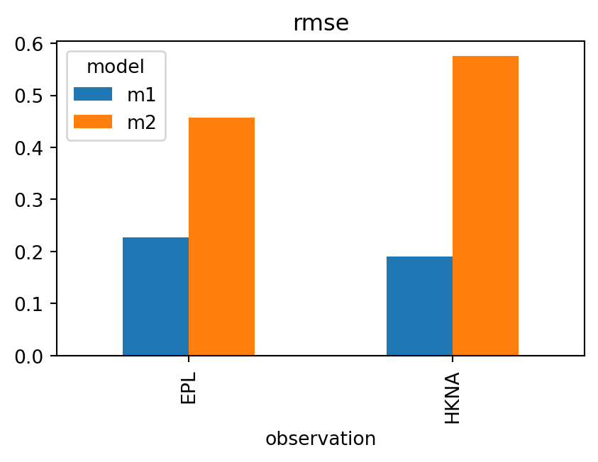
Example 11: Plotting a bar chart for RMSE
= (5 ,3 ))
This creates a bar chart showing RMSE values for each model-observation pair.
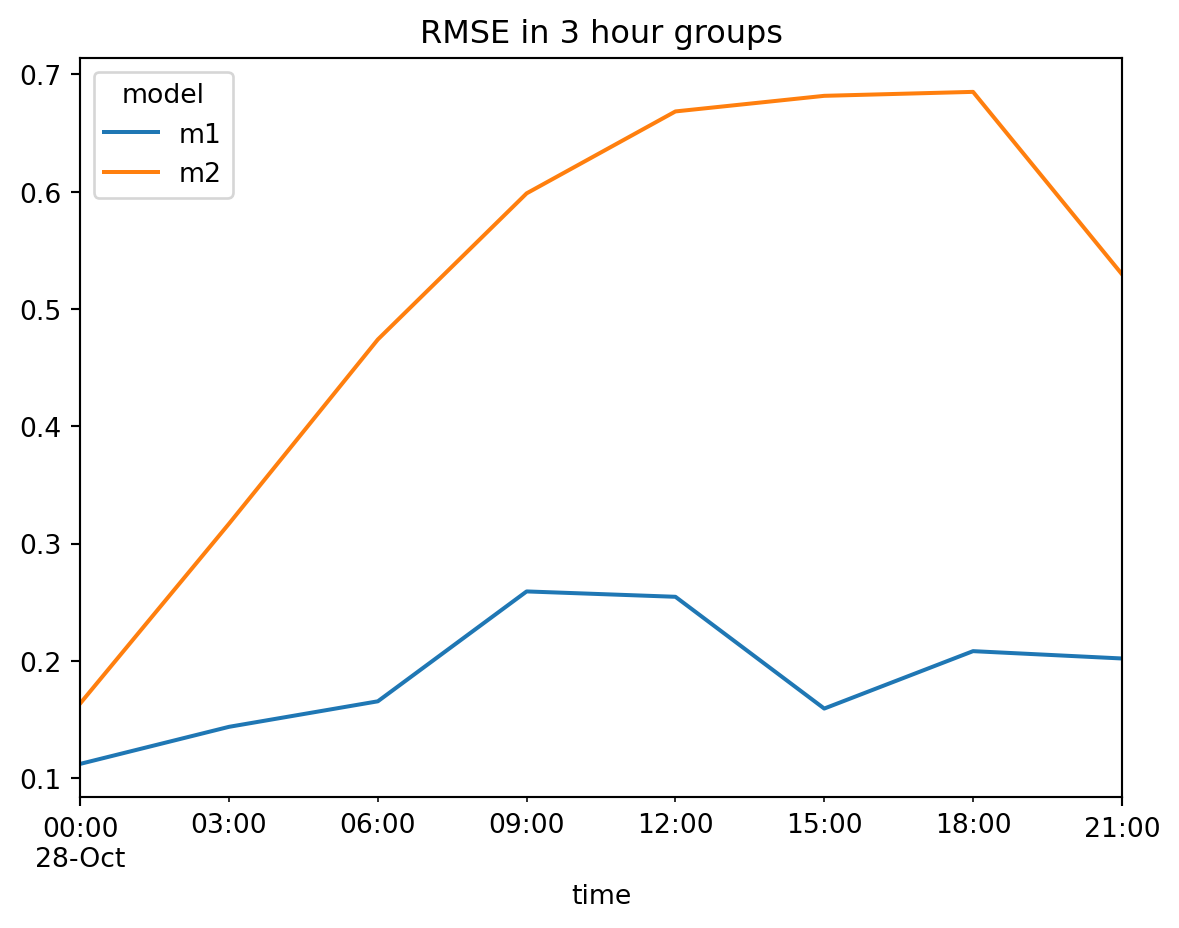
Example 12: Line plot
= cc.skill(by= ['model' ,'freq:3h' ])= "RMSE in 3 hour groups" )
This generates a line plot showing RMSE values over the index.
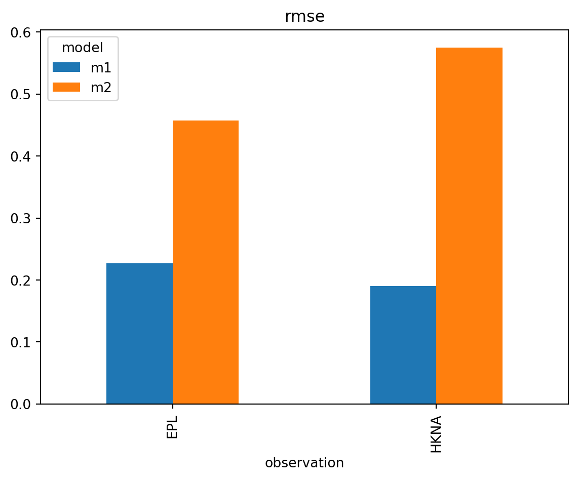
Example 13: Bar chart
This creates a bar chart showing RMSE values for each model-observation pair.
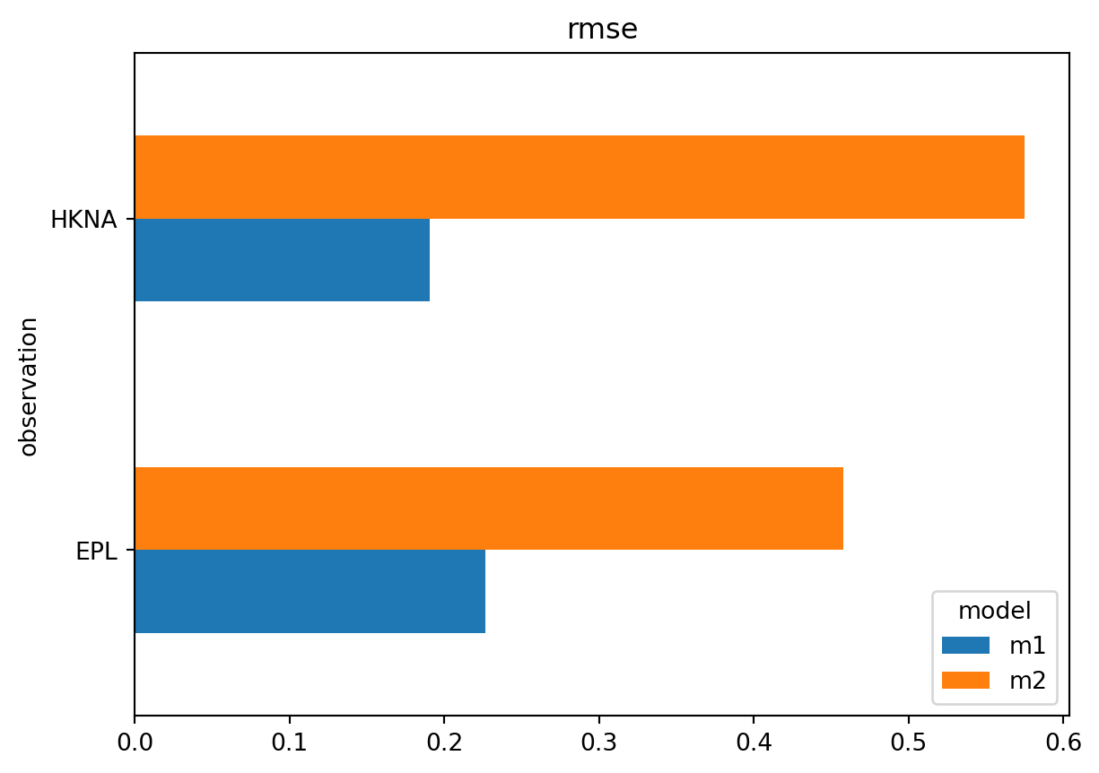
Example 14: Horizontal bar chart
This generates a horizontal bar chart for RMSE values.
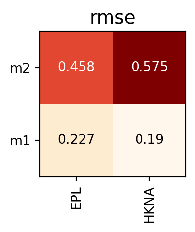
Example 15: Colored grid
This produces a colored grid representation of the skill metrics, which can help identify patterns.
Exporting a SkillTable
For further analysis, the SkillTablepandas.DataFrame
Example 16: Converting to DataFrame
= sk.to_dataframe()
model
observation
m1
HKNA
120
-0.076142
0.190451
0.060252
EPL
22
-0.190022
0.226535
0.049538
m2
HKNA
120
-0.525915
0.574975
0.080212
EPL
22
-0.428523
0.457555
0.064425
This converts the SkillTablepandas.DataFrame
Example 17: Converting to GeoDataFrame
= sk.to_geodataframe()This converts the table to a GeoDataFrame
Summary of Key Methods
The SkillTable
sel()query()sort_index()sort_values()swaplevel()round()plot.line()plot.bar()plot.barh()plot.grid()style()to_dataframe()pandas.DataFrame.to_geodataframe()GeoDataFrame for spatial analysis.
By combining these methods, you can analyze model performance in detail, identify trends, and communicate results effectively.
