Vertical profile

Show a vertical profile dfsu on a map, mark positions along it and subset it by distance.

A vertical profile (2DV) dfsu is a transect with depth, typically written by a MIKE 3 model. This example places a profile on the model domain, marks points of interest along it, and cuts out part of it.

import matplotlib.pyplot as plt
import numpy as np

import mikeio

Profile on the model domain

ds = mikeio.read("../../data/oresund_vertical_slice.dfsu")
g = ds.geometry
model_domain = mikeio.open("../../data/oresundHD_run1.dfsu").geometry

_, ax = plt.subplots(1, 2, figsize=(12, 4))
model_domain.plot(ax=ax[0], title="Transect")
g.plot(color="r", ax=ax[0])
g.plot.mesh(ax=ax[1], title="Transect mesh");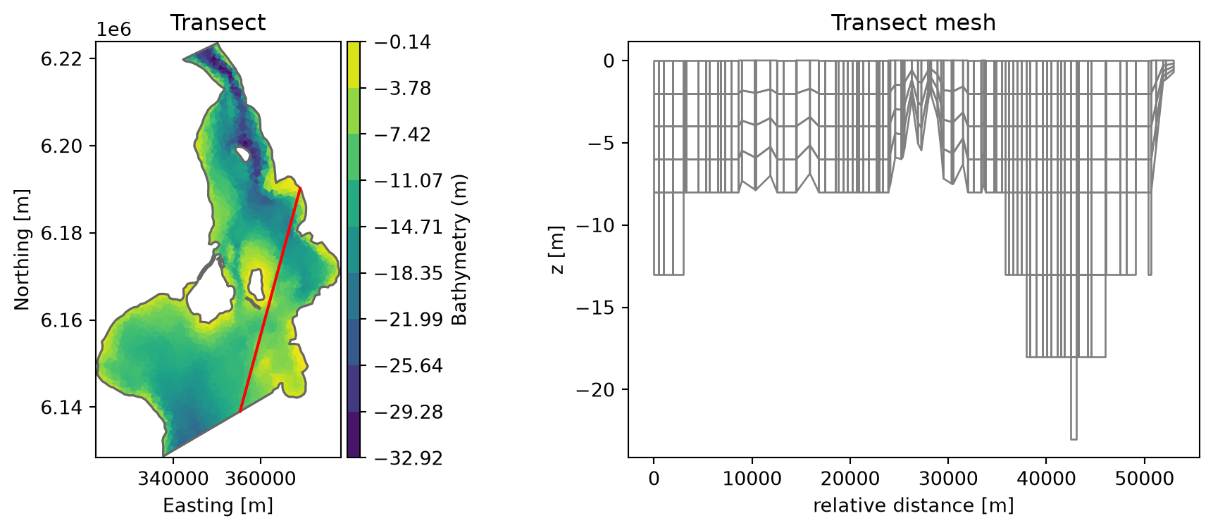

Marking positions along the profile

The x-axis of a profile plot is the distance along the transect. get_nearest_relative_distance converts a map position to that distance, so points of interest can be marked on both plots:

ptA = (3.55e05, 6.145e06)
ptB = (3.62e05, 6.166e06)
distA = g.get_nearest_relative_distance(ptA)
distB = g.get_nearest_relative_distance(ptB)

_, ax = plt.subplots(1, 2, figsize=(12, 4))
model_domain.plot(ax=ax[0], title="Transect")
g.plot(color="r", ax=ax[0])
for pt, dist, label in [(ptA, distA, "A"), (ptB, distB, "B")]:
    ax[0].plot(*pt, color="b", marker="*", markersize=10)
    ax[1].axvline(dist, color="0.5")
    ax[1].text(dist + 500, -20, f"position {label}")
ds["Temperature"].isel(time=2).plot(ax=ax[1]);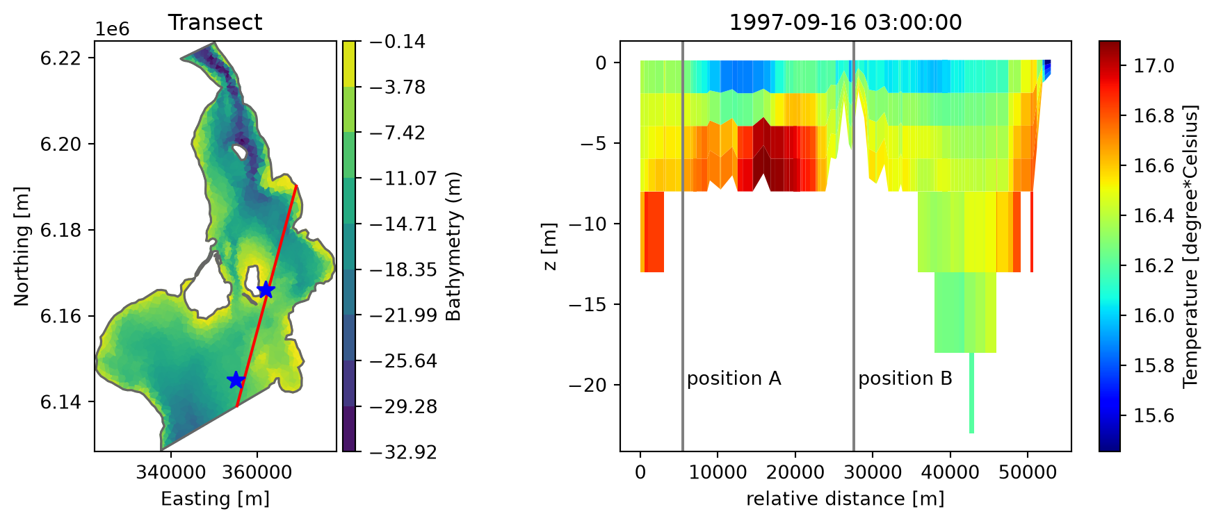

Subsetting by distance

relative_element_distance holds the distance of each element along the profile. Select the part between 10 and 25 km:

rd = g.relative_element_distance
idx = np.where((rd > 10_000) & (rd < 25_000))[0]
ds_sub = ds.isel(element=idx)
ds_sub["Temperature"].isel(time=-1).plot();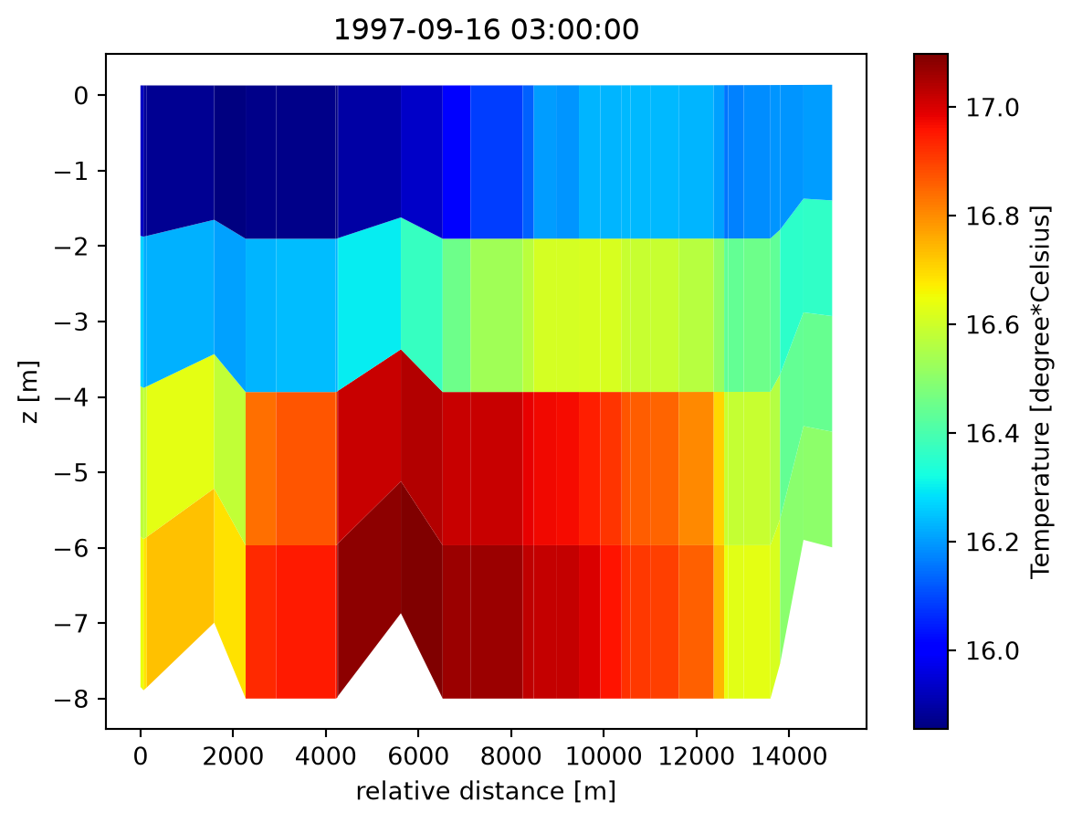

A bent profile in geographical coordinates

A profile need not be straight. This one follows a curved path near Kalundborg, in longitude/latitude:

ds = mikeio.read("../../data/kalundborg_transect.dfsu")
model_domain = mikeio.open("../../data/kalundborg_coarse.mesh").geometry

ax = model_domain.plot.outline()
ds.geometry.plot(color="cyan", ax=ax);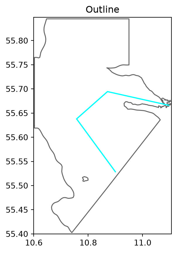

ds["U velocity"].isel(time=-1).plot(figsize=(12, 4));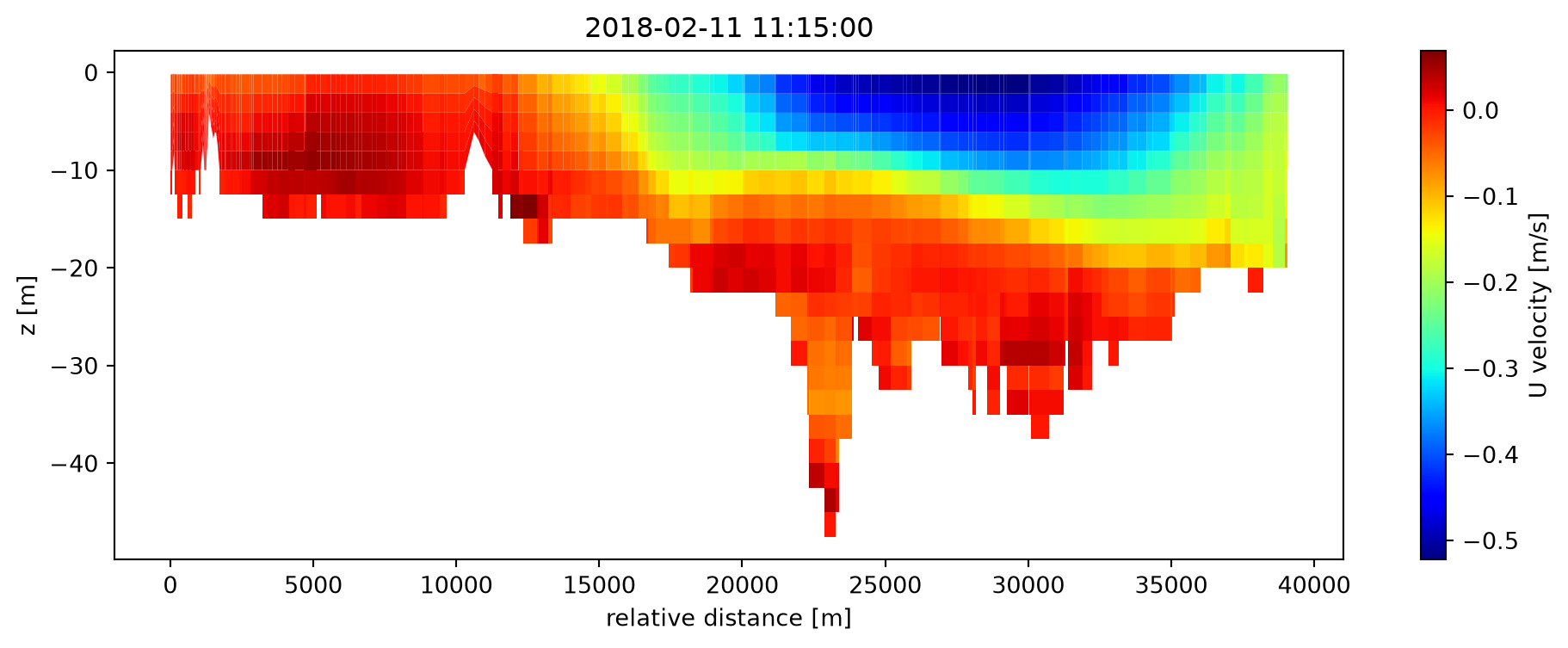

A single column, one line per time step:

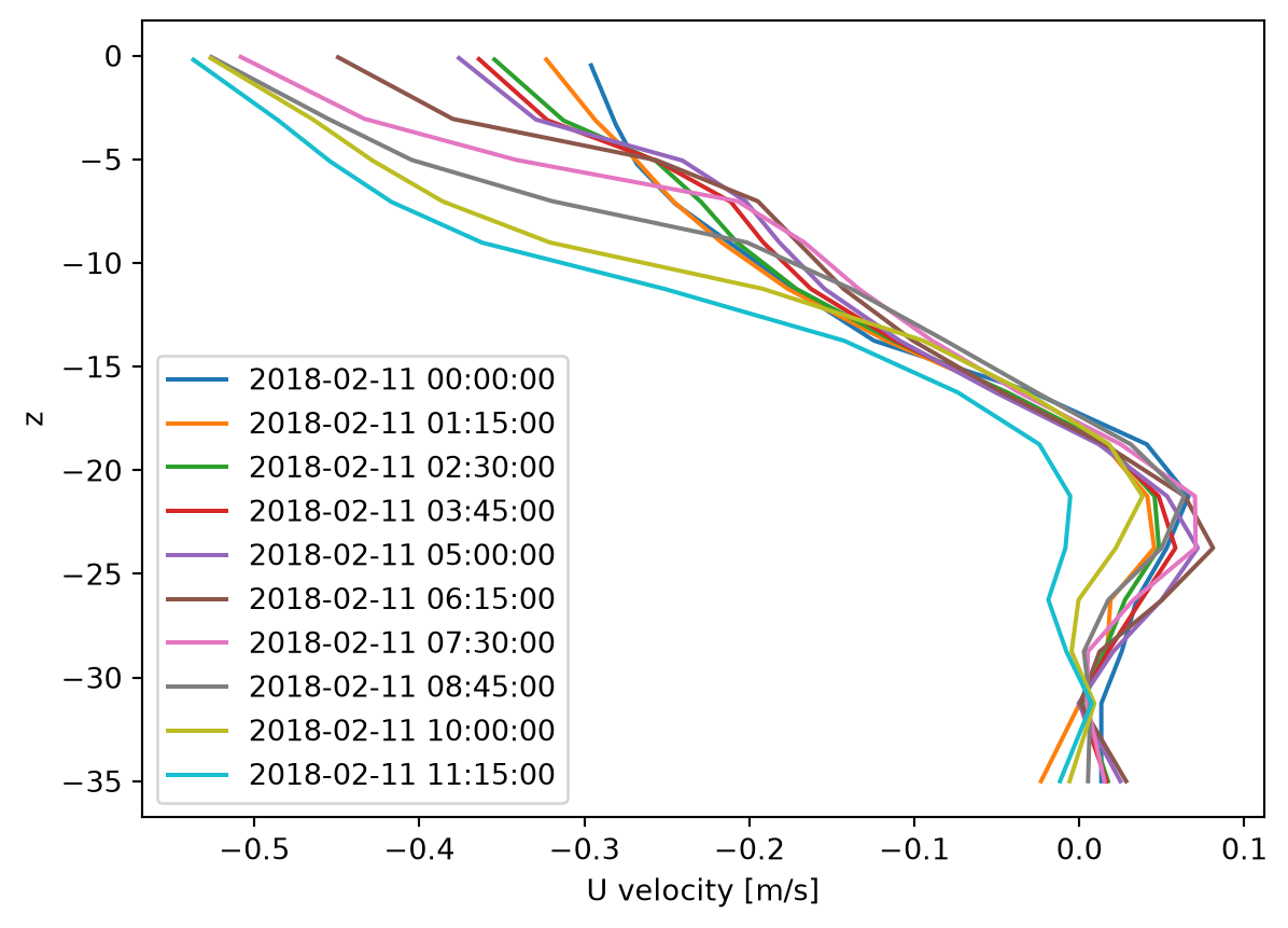
ds.sel(x=10.8, y=55.6)["U velocity"].plot()
plt.legend(ds.time);