CMEMS to vertical profile

Convert Copernicus Marine (CMEMS) gridded data to a MIKE dfsu vertical profile.

This example shows how to extract a vertical transect from a Copernicus Marine (CMEMS) NetCDF file and save it as a dfsu vertical profile — an unstructured mesh format commonly used as boundary conditions in MIKE hydrodynamic models.

Setup

import numpy as np
import xarray as xr
import matplotlib.pyplot as plt

import mikeio
from mikeio.spatial import GeometryFMVerticalProfile
from mikecore.DfsuFile import DfsuFileType

Load CMEMS data

This example uses a small Baltic Sea subset downloaded with the Copernicus Marine Toolbox:

ds_cmems = xr.open_dataset("../../data/cmems_mod_bal_phy_anfc_P1D.nc")
ds_cmems

Define a transect

Define a transect as evenly-spaced points between two endpoints, using the native grid resolution.

lon_start, lat_start = 23.6, 59.3
lon_end, lat_end = 23.6, 59.6
n_points = 20

transect_lon = np.linspace(lon_start, lon_end, n_points)
transect_lat = np.linspace(lat_start, lat_end, n_points)

fig, ax = plt.subplots()
ds_cmems["thetao"].isel(time=0, depth=0).plot(ax=ax)
ax.plot(transect_lon, transect_lat, "k-o", markersize=3, label="Transect")
ax.legend()
ax.set_title("Surface temperature with transect");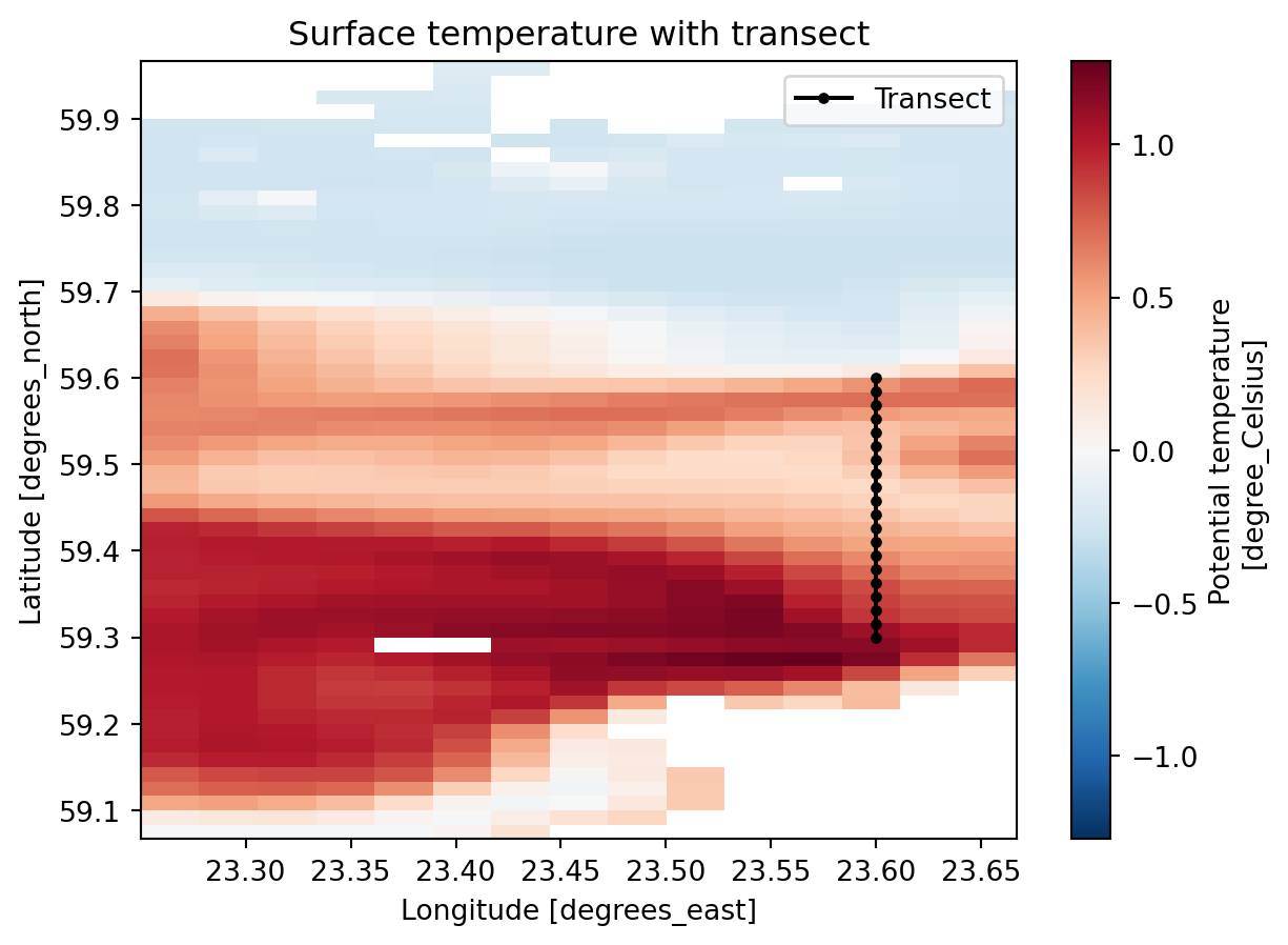

Extract data along the transect

Select the nearest grid point for each transect position using xarray.

ds_transect = ds_cmems.sel(
    latitude=xr.DataArray(transect_lat, dims="points"),
    longitude=xr.DataArray(transect_lon, dims="points"),
    method="nearest",
)

depth = ds_cmems.depth.values
time = ds_cmems.time.values
n_times = len(time)
n_depths = len(depth)

ds_transect

Build the vertical profile mesh

CMEMS data values are cell-centered — each (depth, point) is an element value. The nodes sit at the boundaries between cells.

Nodes

Compute node positions at the interfaces between depth levels and between horizontal points.

# Vertical interfaces: surface, midpoints between levels, bottom
z_interfaces = np.concatenate(
    [[0], (depth[:-1] + depth[1:]) / 2, [depth[-1] + (depth[-1] - depth[-2]) / 2]]
)

# Horizontal interfaces: half-cell before first, midpoints, half-cell after last
half_dlon = (transect_lon[1] - transect_lon[0]) / 2
half_dlat = (transect_lat[1] - transect_lat[0]) / 2
lon_interfaces = np.concatenate(
    [[transect_lon[0] - half_dlon], (transect_lon[:-1] + transect_lon[1:]) / 2, [transect_lon[-1] + half_dlon]]
)
lat_interfaces = np.concatenate(
    [[transect_lat[0] - half_dlat], (transect_lat[:-1] + transect_lat[1:]) / 2, [transect_lat[-1] + half_dlat]]
)

n_nodes_per_col = n_depths + 1

# Build node coordinates: column-major, bottom-to-top
node_coords = np.column_stack([
    np.repeat(lon_interfaces, n_nodes_per_col),
    np.repeat(lat_interfaces, n_nodes_per_col),
    np.tile(-z_interfaces[::-1], n_points + 1),
])

Elements

Each CMEMS cell maps to one element. Skip cells with NaN (below seafloor).

# Seafloor mask: NaN marks cells below the seabed (any variable works, all share the same mask)
mask = ds_transect["so"].isel(time=0).values

# Build full grid of (point, layer) indices, then mask out seafloor
pi_all = np.repeat(np.arange(n_points), n_depths)
li_all = np.tile(np.arange(n_depths), n_points)
di_all = n_depths - 1 - li_all  # depth index (deepest first in mesh)
valid = ~np.isnan(mask[di_all, pi_all])
pi_valid, li_valid, di_valid = pi_all[valid], li_all[valid], di_all[valid]

# Node indices for each quad element: [bottom-left, bottom-right, top-right, top-left]
bl = pi_valid * n_nodes_per_col + li_valid
element_table = [
    np.array([b, b + n_nodes_per_col, b + n_nodes_per_col + 1, b + 1])
    for b in bl
]

Geometry

geometry = GeometryFMVerticalProfile(
    node_coordinates=node_coords,
    element_table=element_table,
    projection="LONG/LAT",
    # SigmaZ allows variable number of layers per column (bottom-following)
    dfsu_type=DfsuFileType.DfsuVerticalProfileSigmaZ,
    # n_layers is the max number of layers in any column
    n_layers=n_depths,
    # n_sigma=1 means only the top layer is guaranteed everywhere;
    # deeper layers are z-layers that can be absent in shallow columns
    n_sigma=1,
)
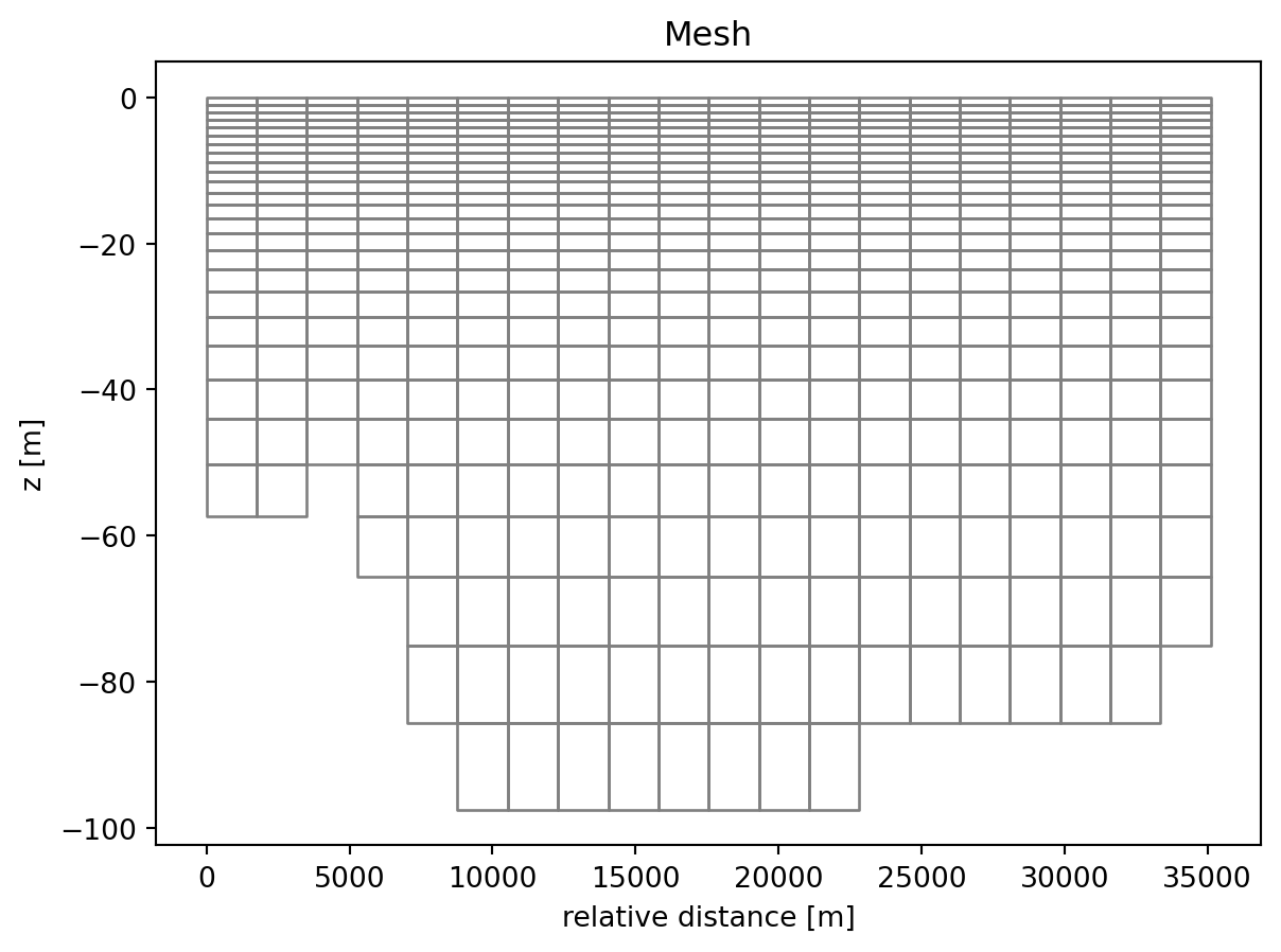
geometry

Flexible Mesh Geometry: DfsuVerticalProfileSigmaZ
number of nodes: 630
number of elements: 515
number of layers: 29
number of sigma layers: 1
projection: LONG/LAT

Write

zn = np.tile(node_coords[:, 2], (n_times, 1)).astype(np.float32)

variables = {
    "thetao": mikeio.ItemInfo("Temperature", mikeio.EUMType.Temperature),
    "so": mikeio.ItemInfo("Salinity", mikeio.EUMType.Salinity),
}

ds_dfsu = mikeio.Dataset([
    mikeio.DataArray(
        data=ds_transect[name].values[:, di_valid, pi_valid],
        time=time, geometry=geometry, item=item, zn=zn,
    )
    for name, item in variables.items()
])
ds_dfsu.to_dfs("transect.dfsu")

Result

ds_back = mikeio.read("transect.dfsu")
ds_back

<mikeio.Dataset>
dims: (time:3, element:515)
time: 2026-03-01 00:00:00 - 2026-03-03 00:00:00 (3 records)
geometry: DfsuVerticalProfileSigmaZ (515 elements, 630 nodes)
items:
  0:  Temperature <Temperature> (degree Celsius)
  1:  Salinity <Salinity> (PSU)

ds_back["Temperature"].isel(time=0).plot();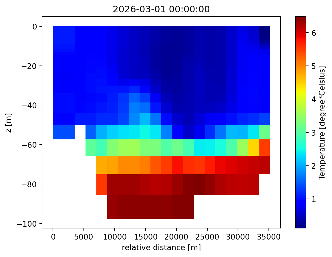

ds_back.geometry.plot.mesh();